


1. Introduction
Lateral movement of the ball, during its trajectory, is one of the tricks used by a bowler to deceive the batsmen in the game of cricket. Two common bowling techniques to generate lateral movement are ‘spin’ and ‘swing.’ The bowler imparts spin to the ball causing it to undergo a sharp deviation when it bounces off the pitch. A spinning ball can also ‘drift’ in the air due to the Magnus effect (Swanson Reference Swanson1961). Spin bowlers usually deliver balls at relatively low speeds (70–90 km h $^{-1}$). Swing bowling, on the other hand, involves deliveries at relatively high speed (>90 km h $^{-1}$). A skillful bowler maintains the angle at which the seam of the ball is oriented with respect to the incoming flow, during its flight. The seam acts as a boundary layer trip. The asymmetry in its orientation results in a lateral aerodynamic force on the ball causing it to swing.
The outer surface of a cricket ball, used in competitive games at the highest level, is made with four pieces of leather. Two quarters are stitched internally to form a hemisphere. The two resulting hemispheres are joined with six rows of stitches that form a prominent ‘seam.’ The outer surface is well polished to result in a smooth finish. Lower quality balls, used for practice and in a lower level of competitions, are manufactured using two pieces of leather. Compared with the four-piece ball, the two-piece ball has stronger departure from sphericity and is less durable. It is generally believed that a bowler has relatively more control on the swing of a four-piece ball. There have been a number of studies in the past to understand the phenomenon of swing (Barton Reference Barton1982; Bentley et al. Reference Bentley, Varty, Proudlove and Mehta1982; Sherwin & Sproston Reference Sherwin and Sproston1982; Mehta et al. Reference Mehta, Bentley, Proudlove and Varty1983; Mehta Reference Mehta1985, Reference Mehta2014; Deshpande, Shakya & Mittal Reference Deshpande, Shakya and Mittal2018; Shah, Shakya & Mittal Reference Shah, Shakya and Mittal2019).
Several factors influence the swing force experienced by the ball and, therefore, its trajectory. Some of them are the weather conditions, orientation of the seam with respect to the incoming flow (Mehta Reference Mehta1985; Deshpande et al. Reference Deshpande, Shakya and Mittal2018), condition of the ball including its surface roughness (Mehta Reference Mehta2014; Shah et al. Reference Shah, Shakya and Mittal2019), speed of the ball and its rate of rotation due to the backspin imparted by the bowler (Mehta Reference Mehta2014). Lateral movement of the ball in the direction of the seam is referred to as conventional swing (CS). Under certain conditions, the ball can move away from the direction of the seam. This is referred to as reverse swing (RS). Deshpande et al. (Reference Deshpande, Shakya and Mittal2018) showed that a new ball undergoes CS at moderate to high (90–145 km h $^{-1}$) and RS at relatively high speed (>145 km h $^{-1}$). Another ploy to manipulate the lateral movement of the ball is via a ‘contrast swing.’ As the game progresses, the bowling side allows one half of the ball to gain natural roughness while continually polishing the other half (Mehta Reference Mehta2014). Deshpande et al. (Reference Deshpande, Shakya and Mittal2018) and Shah et al. (Reference Shah, Shakya and Mittal2019) conducted wind-tunnel experiments to investigate the effect of relative roughness of the two halves of the ball as well as the seam on the swing.
A cricket ball can be modelled as a sphere with boundary layer trip. Uniform flow past a smooth sphere has been extensively studied in the past. The key parameter is the Reynolds number defined as  $Re = U D/ \nu$, where $U$ is the free-stream speed of the incoming flow, $D$ is the diameter of the sphere and $\nu$ is the kinematic viscosity of the fluid. Based on the variation of the mean drag coefficient with $Re$, Achenbach (Reference Achenbach1972) classified the flow into four regimes: subcritical, critical, supercritical and transcritical. The boundary layer separates in a laminar state in the subcritical regime and does not reattach. The separated boundary layer transitions to a turbulent state in the critical regime, causing it to reattach. A laminar separation bubble (LSB) forms delaying the final separation (Fage Reference Fage1936; Raithby & Eckert Reference Raithby and Eckert1968; Achenbach Reference Achenbach1972; Taneda Reference Taneda1978; Deshpande et al. Reference Deshpande, Shakya and Mittal2018) and leading to a narrower wake and a significant decrease in drag, often referred to as drag crisis. The boundary layer transitions to a turbulent state prior to its separation in the supercritical regime, without the formation of a LSB. In the transcritical regime the transition point is located upstream of the shoulder ( $\phi = 90^\circ$, see figure 1) and moves further upstream, towards the stagnation point, with an increase in $Re$. The drag coefficient increases with an increase in $Re$ in this regime (Achenbach Reference Achenbach1972).

Figure 1. A view of the ball illustrating the seam and definition of  $\theta$ (polar) and $\phi$ (azimuthal) angles. Free-stream flow is along the $x$ axis.
The LSB and the associated drag crisis has also been observed for a circular cylinder (Roshko Reference Roshko1954; Tani Reference Tani1964; Achenbach & Heinecke Reference Achenbach and Heinecke1981; Schewe Reference Schewe1983; Williamson Reference Williamson1996; Singh & Mittal Reference Singh and Mittal2005a; Lehmkuhl et al. Reference Lehmkuhl, Rodríguez, Borrell, Chiva and Oliva2014; Rodríguez et al. Reference Rodríguez, Lehmkuhl, Chiva, Borrell and Oliva2015; Cheng et al. Reference Cheng, Pullin, Samtaney, Zhang and Gao2017; Chopra & Mittal Reference Chopra and Mittal2017, Reference Chopra and Mittal2022b). Chopra & Mittal (Reference Chopra and Mittal2022b), from their large eddy simulation (LES), reported a secondary vortex (SV) in addition to the LSB. The SV forms in the low subcritical regime while the LSB appears in the critical regime. Both coexist in the critical and supercritical regimes with the SV lying between the LSB and surface of the cylinder. The LSB is associated with a plateau in the pressure distribution on the surface of the cylinder, while the SV leads to a sharp dip followed by a recovery, resembling a ‘kink.’
The effect of a trip wire on the flow past a sphere was investigated by Maxworthy (Reference Maxworthy1969) and Son et al. (Reference Son, Choi, Jeon and Choi2011). The experiments in the study by Son et al. (Reference Son, Choi, Jeon and Choi2011) were carried out in a wind tunnel. The trip wire traces a circle on the surface of the sphere and is placed in an axisymmetric manner such that the azimuthal angle of each point on the trip, with respect to the front stagnation point on the sphere, is the same. Compared with a smooth sphere, the drag crisis with a trip wire occurs at a lower  $Re$. A trip wire of size smaller than the thickness of the boundary layer causes delayed laminar separation, transition of the separated shear layer and its subsequent reattachment. A LSB forms between the points of laminar separation and turbulent reattachment. Son et al. (Reference Son, Choi, Jeon and Choi2011) found a similar flow structure. However, they referred to it as the secondary separation bubble. A trip wire of thickness larger than the thickness of the boundary layer causes direct transition to turbulence without the formation of a LSB. Igarashi (Reference Igarashi1986) conducted a similar experimental study for a circular cylinder. It was found that the flow downstream of the trip may either: (i) relaminarize, (ii) transition to a turbulent state and reattach as a turbulent boundary layer, or (iii) remain separated with no further reattachment depending on the $Re$ and the size and location of the trip. Chopra & Mittal (Reference Chopra and Mittal2022a) conducted LES for a circular cylinder with a trip of various height placed in the region of favourable pressure gradient at $55^\circ$ from the front stagnation point. Natural transition, via formation of a LSB, albeit at lower $Re$ compared with that for a smooth cylinder, was observed for a trip of height $0.25\,\%$ of the diameter of the cylinder. Direct transition, where the formation of a LSB is bypassed, was reported for a trip of height $1\,\%$ of the cylinder diameter. The drag crisis in both cases is in two stages. The effect of the trip is experienced by the non-trip side as well. A relatively large reverse lift is observed during the second stage of drag crisis.
The seam introduces disturbance in the boundary layer on the seam side of a cricket ball. The asymmetry of surface pressure on the seam and the non-seam sides causes the cricket ball to swing (Mehta et al. Reference Mehta, Bentley, Proudlove and Varty1983; Mehta Reference Mehta1985). Deshpande et al. (Reference Deshpande, Shakya and Mittal2018) carried out oil-flow visualization and force and surface pressure measurements in a low-turbulence wind tunnel to understand the role of the seam in the swing of a cricket ball. Experiments were conducted for various flow speeds and several orientations of the seam to the flow. It was found that the seam does not have a significant effect on the flow at relatively low  $Re$. A LSB forms on the seam side of the ball beyond a certain $Re$ leading to CS. It is localized to a specific region on the seam side due to the varying azimuthal location of the seam relative to the stagnation point. At other azimuthal locations, the boundary layer either separates in a laminar state with further reattachment, or directly transitions to a turbulent state with the formation of a LSB. The region of direct transition increases, while the size of the LSB shrinks, with an increase in $Re$. The boundary layer on the non-seam side undergoes a transition beyond a certain $Re$. The transition point, on both the seam and non-seam sides, moves upstream with an increase in $Re$. It moves upstream of the seam, on the seam side, beyond a certain $Re$ causing the boundary layer to thicken once it encounters the seam (Mehta Reference Mehta2005). As a result, the final separation point of the boundary layer on the seam side is relatively upstream compared with that on the non-seam side. The higher suction on the non-seam side causes the ball to undergo RS. The formation of the LSB during RS was also reported by Scobie et al. (Reference Scobie, Pickering, Almond and Lock2012).
It was shown by Kim et al. (Reference Kim, Choi, Park and Yoo2014) that a spinning sphere may experience a lateral force, in the plane normal to the axis of spin, due to the Magnus or inverse Magnus effect. Most swing bowlers in cricket release the ball along the seam (Mehta Reference Mehta1985). Except for deliveries from bowlers with a side-arm action, the axis of the backspin of the ball at its release is close to horizontal and normal to the plane of the seam. Therefore, the force because of spin of the ball is vertically upwards due to the Magnus effect. It is downwards if the flow is in the regime of inverse Magnus effect. In contrast, the swing force is in the lateral direction that is almost normal to the plane containing the seam of the ball. As a result, the Magnus/inverse Magnus force is not expected to directly contribute to the lateral movement of the ball. However, the rotation of the ball has some effect on the pressure distribution on its surface. Barton (Reference Barton1982) showed that the magnitude of swing force on the ball decreases with an increase in rotation rate. The primary objective of the present study is to understand the role of the seam on the swing of a cricket ball. Therefore, the effect of rotation of the ball is not explored in this work. All computations are carried out for a non-spinning model of a cricket ball. A similar approach was undertaken by Deshpande et al. (Reference Deshpande, Shakya and Mittal2018) in their wind-tunnel experiments.
Deshpande et al. (Reference Deshpande, Shakya and Mittal2018) reported the variation of the time-averaged swing force coefficient ( $\bar {C}_z$) with $Re$ for a new cricket ball as well as its three-dimensional (3-D) printed model. Despite the polishing, the new cricket ball has higher surface roughness compared with the 3-D printed model. In addition, the secondary seam as well as the embossing of the logo of the manufacturer contribute to the surface roughness and spatial inhomogeneity of a cricket ball. To distinguish between the two articles, the 3-D printed model is referred to as a sphere with five trips. The variation of force coefficients with $Re$ is qualitatively similar for both models. However, the critical $Re$ for onset of CS and transition from CS to RS is significantly lower for the new cricket ball ( $Re_{critical} \approx 1.8 \times 10^5$) compared with that for the sphere with five trips ( $Re_{critical} \approx 3.2 \times 10^5$). The $Re_{critical}$ for transition from CS to RS for a cricket ball is expected to be significantly affected by the quality of leather, embossing of the manufacturer's logo and the variations in the manufacturing process. The data for the seam orientation of $30^\circ$ to the incoming flow is especially relevant to the present work. For the sphere with five trips, $\bar {C}_z$ is close to zero for $Re$ less than $0.5 \times 10^5$, approximately. This range of $Re$ is referred to as the regime of no swing (NS). Here $\bar {C}_z$ gradually increases at the onset of the CS regime and saturates to a value of close to $0.35$ at $Re \sim 1.6 \times 10^5$. It stays constant at this value up to $Re \sim 3.2 \times 10^5$ where it undergoes a steep reversal to $\bar {C}_z=-0.05$ approximately, marking the onset of the RS regime. Deshpande et al. (Reference Deshpande, Shakya and Mittal2018) and Scobie et al. (Reference Scobie, Pickering, Almond and Lock2012) attributed the CS to the transition of the boundary layer to a turbulent state on the seam side of the cricket ball. This, however, does not explain the gradual increase in $\bar {C}_z$ at the onset of the CS. According to Deshpande et al. (Reference Deshpande, Shakya and Mittal2018), the transition of the boundary layer on the seam side is accompanied with the formation of a LSB. It is generally believed that once formed, the streamwise extent of the LSB decreases with an increase in $Re$. If formation of the LSB is indeed the reason for the CS, $\bar {C}_z$ should experience an abrupt increase at the onset of the regime and gradually decrease with an increase in $Re$. This prompts further exploration of the possible mechanism of the CS to explain the gradual increase of swing force coefficient in the early stage of the CS regime.
The flow past a sphere with five trips is investigated through LES for  $5 \times 10^4 \leq Re \leq 4.5 \times 10^5$. The study addresses the following specific questions. (i) How does the seam affect the transition of the boundary layer? (ii) Why does the swing force coefficient show a gradual increase in the initial part of the CS regime? (iii) What are the various vortex structures associated with the flow during CS and RS? (iv) How do the LSB and SV on the seam and non-seam sides evolve with an increase in $Re$? The force coefficients from the computations are compared with those reported earlier from wind-tunnel measurements. To enable comparison, the same nomenclature proposed by Deshpande et al. (Reference Deshpande, Shakya and Mittal2018) for problem set-up and analysis of data is followed.
The seam angle considered in this work is  $30^\circ$ (see figure 1). It enables comparison with the force and surface pressure measurements as well as oil-flow visualization experiments carried out by Deshpande et al. (Reference Deshpande, Shakya and Mittal2018) for this seam angle in a wind tunnel. Force measurements for several seam angles have also been carried out by Shah & Mittal (Reference Shah and Mittal2023) with the objective to investigate the possibility of a knuckleball delivery in cricket, inspired from that in baseball.
2. Computational details
2.1. The governing equations
The equations that govern an incompressible flow are as follows:
 \begin{gather} \left(\frac{\partial\boldsymbol{u}}{\partial t} + \boldsymbol{u}\boldsymbol{\cdot}\boldsymbol{\nabla} \boldsymbol{u}\right) - \boldsymbol{\nabla}\boldsymbol{\cdot}\boldsymbol{\sigma} = 0 \quad \text{on}\ \boldsymbol{\varOmega} \times (0,t) , \end{gather}
 \begin{gather}\boldsymbol{\nabla}\boldsymbol{\cdot} \boldsymbol{u} = 0 \quad \text{on}\ \boldsymbol{\varOmega} \times (0,t) . \end{gather}
Here  $\rho$ is the density of the fluid, $\boldsymbol {u}$ is the velocity vector and $\boldsymbol {\sigma }$ is the stress tensor. The stress tensor for a Newtonian fluid is $\boldsymbol {\sigma } = -p\boldsymbol {I} + 2\mu \boldsymbol {\epsilon }(\boldsymbol {u})$, where p is the pressure, $\mu$ is the coefficient of viscosity of the fluid and $\boldsymbol {\epsilon }$ is the strain-rate tensor defined as $\boldsymbol {\epsilon } = \frac {1}{2}((\boldsymbol {\nabla }\boldsymbol {u}) + (\boldsymbol {\nabla }\boldsymbol {u})^{\rm T})$.
A stabilized finite element method is utilized to solve these equations. Very fine grids are utilized close to the surface of the body to resolve the boundary layers, their separation and transition. Owing to the large Reynolds number of the flows considered in the study, and the constraint of the available computational resources, it is not possible to carry out direct numerical simulation to resolve all the flow scales including those in the wake. Therefore, LES is carried out. The sigma turbulence model (Nicoud et al. Reference Nicoud, Toda, Cabrit, Bose and Lee2011) is used to model the subgrid scales in the flow. Similar to the work of Johari & Stein (Reference Johari and Stein2002), the turbulence model is implemented by replacing the molecular viscosity,  $\mu$, by the sum of the molecular and eddy viscosity ( $=\mu + \mu _{SGS}$) in the equation representing the constitutive model. The eddy viscosity for the sigma sub-grid scale model is defined as $\mu _{SGS} = (C_m \varDelta )^2({\varPi _3(\varPi _1 - \varPi _2)(\varPi _2 - \varPi _3)}/{\varPi _1^2})$. The value of the model constant, $C_m$, is $1.35$ as proposed by Nicoud et al. (Reference Nicoud, Toda, Cabrit, Bose and Lee2011). Here $\varDelta$ is the sub-grid characteristic length scale and $\varPi _1,\varPi _2,\varPi _3$ are the singular values of the velocity gradient tensor. The model in conjunction with LES has been used in our earlier work for investigating drag crisis on a circular cylinder with and without a boundary layer trip (Chopra & Mittal Reference Chopra and Mittal2022a,Reference Chopra and Mittalb).
2.2. The finite element formulation
All computations are carried out using a stabilized finite element formulation (Tezduyar et al. Reference Tezduyar, Mittal, Ray and Shih1992) of the equations governing the fluid flow. The stabilization is via the streamline-upwind/Petrov–Galerkin (SUPG), pressure-stabilizing/Petrov–Galerkin (PSPG) and least-squares terms based on the incompressibility constraint (LSIC). Galerkin formulation is known to result in node-to-node oscillations in the velocity field for flows dominated by advection. Inclusion of SUPG terms renders stability to the formulation. The PSPG terms allow one to use a certain combination of pressure–velocity interpolation functions that do not work with the Galerkin formulation, including equal-in-order interpolation. The LSIC terms are effective in stabilizing the computations against oscillations that might appear in simulations at relatively large  $Re$. The second-order-accurate-in-time, Crank–Nicholson scheme is utilized for time integration. The algebraic equation systems resulting from the finite element discretization of the flow equations are solved using the matrix-free generalized minimal residual technique (Saad & Schultz Reference Saad and Schultz1986) in conjunction with diagonal preconditioners. The formulation is implemented on a distributed memory parallel system (Behara & Mittal Reference Behara and Mittal2009). Message passing interface libraries have been used for inter-processor communication. The same computational set-up has been successfully applied to solve various flow problems in the past (Tezduyar et al. Reference Tezduyar, Mittal, Ray and Shih1992; Singh & Mittal Reference Singh and Mittal2005b; Chopra & Mittal Reference Chopra and Mittal2017; Pandi & Mittal Reference Pandi and Mittal2019; Chopra & Mittal Reference Chopra and Mittal2022a).
2.3. Problem set-up
The cricket ball is modelled by a sphere of diameter  $D$ with five trip wires placed on its surface, as shown in figure 1. This geometry is similar to that used by Deshpande et al. (Reference Deshpande, Shakya and Mittal2018) in their experiments for a sphere with five trips. The trip wires collectively model the seam of a cricket ball. The central trip, lying on the equatorial plane of the sphere and with a height corresponding to $1.4\,\%$ of $D$, is the tallest and is referred to as the major seam. It is flanked by two minor seams on either side. The height of each minor seam is $0.49\,\%$ of $D$. Figure 1 also shows the polar and azimuthal angles that are referred to later in the paper while discussing the results. The $x$–
$x$– $z$ plane passing through $y=0$ is referred to as the equatorial plane and the $x$–
$x$– $y$ plane passing through $z=0$ as the polar plane. The seam is oriented at an azimuthal angle of $\phi _T$ to the free stream. All computations in this work are for a seam angle of $\phi _T=30^\circ$.
Figure 2 shows a schematic of the computational domain. The outer boundary of the domain is a hexahedral box. The free-stream flow is along the  $x$ axis. The streamwise extent of the domain is $L_x = 40D$ while its dimension in the cross-stream ( $L_y$) and lateral direction ( $L_z$) is 20D each. The boundary conditions are also marked in the figure. Uniform flow is prescribed on the inflow boundary while the stress vector is assigned zero value at the outlet. A ‘slip wall’ boundary condition is prescribed at the lateral walls of the domain, with the velocity component normal to and the stress component along the boundary of the wall being assigned zero value. The ‘no-slip’ condition is assigned to the velocity on the nodes lying on the surface of the cricket ball.

Figure 2. Schematic of the problem set-up, computational domain and boundary conditions.
2.4. The finite element mesh and convergence study
Figure 3 shows different views of the finite element mesh used in the present study. It consists of 30 million nodes and 80 million elements approximately. This is referred to as mesh M1. Equal-in-order interpolation functions for velocity and pressure are used for spatial discretization. The mesh is a mix of six-noded wedge elements in the inflation layers near the ball and four-noded tetrahedral elements away from it. The mesh near the surface of the ball is sufficiently fine to resolve the boundary layer and its separation for the  $Re$ range considered. The height of the first layer of elements on the surface of the ball, normal to it, is ${\approx } 6 \times 10^{-6}D$. The corresponding value of y $^+$ ( $=yv^*/\nu$), for the highest $Re$ considered in the study ( $= 4.5 \times 10^5$), is 0.13, 0.32 and 0.10 at $\phi = 10^\circ$, 60 $^\circ$ and 100 $^\circ$, respectively. Here, $y$ is the distance of the field point from the surface of the ball and $v^*$ is the wall-friction velocity defined as $v^*=\sqrt {\tau _w / \rho }$, where $\tau _w$ is the shear stress at the wall. It is noted that $y^+$ for all the elements lying on the surface of the cylinder is less than $1$, reflecting the adequacy of the spatial resolution of the mesh in the radial direction close to the surface of the ball.

Figure 3. (a) A sectional view of the finite element mesh M1 on the  $x$–
$x$– $z$ plane at $y = 0$. (b) A close-up view of the surface mesh. The edges of each triangular element are of length $5 \times 10^{-4}D$ approximately. (c) A close-up view of a section of the mesh showing the inflation layers near the surface of the ball. The height of the first layer of elements on the surface is $6 \times 10^{-6}D$.
The adequacy of the resolution of mesh M1 is assessed by carrying out computations on a finer mesh, M2 consisting of  $50$ million nodes and $150$ million elements approximately. To save on resources, computations with mesh M2 have been carried out for one half of the domain by utilizing the symmetry of the geometry about the $x$–
$x$– $z$ plane passing through the centre of the cricket ball. Symmetry conditions, corresponding to the velocity component normal to and the stress component along the plane being assigned zero value, are prescribed on the $x$–
$x$– $z$ plane. Compared with mesh M1, M2 has a larger number of inflation layers near the surface of the ball. The height of the elements normal to the surface of the ball, in the inflation layers, is smaller for mesh M2 compared with mesh M1. Additionally, the surface mesh as well as that in the near wake is finer. Results from the two meshes are compared for $Re=3 \times 10^5$ that is associated with a LSB on the seam side and lies in the CS regime.
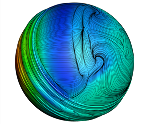
Figure 4 shows the pressure coefficient and surface streamlines for the time-averaged flow obtained with the two meshes. The upper row shows results with mesh M1 while those with M2 are shown in the lower row. The two sets of results are in very good agreement. To enable a quantitative comparison, figure 5 shows the azimuthal variation of the time-averaged coefficient of pressure ( $\bar {C}_P$) on a plane corresponding to a polar angle of $\theta = 5^\circ$. The two sets of results are in excellent agreement. The time-averaged drag and swing force coefficients for mesh M1 are $\bar {C}_D=0.232$ and $\bar {C}_L=0.228$. These values for mesh M2 are $\bar {C}_D=0.228$ and $\bar {C}_L=0.221$. The azimuthal angle on the seam side of the ball, at the equatorial plane corresponding to the reattachment point of the boundary layer in the turbulent state and the end of the LSB, determined from the variation of skin friction on the surface, is $120.6^\circ$ and $121.7^\circ$ for mesh M1 and M2, respectively. The good agreement between the two sets of results confirms the adequacy of mesh M1 to resolve the flow for the range of $Re$ considered in this study. All the results presented in this paper have been computed with mesh M1.

Figure 4. Comparison of the time-averaged flow at  $Re = 3 \times 10^5$ computed on (i) mesh M1 and (ii) mesh M2 (one half of the domain is modelled). (a) Side view (viewed from the positive $y$ axis), (b) top view (viewed from the positive $z$ axis) and (c) bottom view (viewed from the negative $z$ axis) showing the distribution of the coefficient of pressure ( $\bar {C}_P$) on the surface of the ball overlayed with surface streamlines.

Figure 5. Comparison of the time-averaged flow at  $Re = 3 \times 10^5$ computed on (i) mesh M1 and (ii) mesh M2 (one half of the domain is modelled): azimuthal variation of time-averaged coefficient of pressure ( $\bar {C}_P$) at $\theta = 5^\circ$.
3. Results
Computations are carried out for various  $Re$ in the range $5 \times 10^4 \leq Re \leq 4.5 \times 10^5$ to span the regime of NS, CS and RS (Deshpande et al. Reference Deshpande, Shakya and Mittal2018). The seam angle for the study is $\phi _T = 30^\circ$. At each $Re$, time integration of the flow equations is carried out for a sufficiently long time to ensure that the statistics related to the time variation of force coefficients achieves stationarity. Data for at least 30 time units has been utilized to estimate the time averages.
3.1. Overview of the various regimes
Figure 6 shows the variation of the drag and swing force coefficients with Reynolds number. The force coefficients are obtained by non-dimensionalizing the forces, experienced by the sphere with five trips, using free-stream dynamic pressure multiplied with the projected area of the clean sphere without trips. Also shown in the figure are the measurements by Deshpande et al. (Reference Deshpande, Shakya and Mittal2018) from their wind-tunnel experiments for a synthetic model of a cricket ball with a very similar seam configuration. The two sets of results are in reasonable agreement. The regimes of NS, CS and RS classified on the basis of the time-averaged swing force coefficient, from both the studies, are marked in figure 6(b). Also marked are certain features of the flow observed in different regimes. Consistent with the results from Deshpande et al. (Reference Deshpande, Shakya and Mittal2018), it is noted that  $\bar {C}_Z$ is approximately zero for $Re$ up to $5 \times 10^4$ suggesting that the seam does not significantly affect the flow in this range of $Re$. Therefore, $Re \le 5 \times 10^4$ is referred to as the NS regime.

Figure 6. Variation of the time-averaged (a) drag coefficient,  $\bar {C}_D$, and (b) swing coefficient, $\bar {C}_Z$, with Re. Positive values of $\bar {C}_Z$ correspond to CS and negative values correspond to RS. The regimes of NS, CS and RS, based on the present study as well as from the experimental study by Deshpande et al. (Reference Deshpande, Shakya and Mittal2018), are marked in (b). Also marked are flow regimes with respect to the state of the boundary layer.
The boundary layer thickness,  $\delta$, at any azimuthal location decreases with an increase in $Re$. Therefore, the non-dimensional height of the trip, with respect to $\delta$, increases with an increase in $Re$, thereby increasing its effectiveness in introducing a disturbance. An interesting aspect of the seam is that the flow encounters it at varying azimuthal angle, with respect to the front stagnation point, at each polar plane (see figure 1). While the seam is in the zone of favourable pressure gradient in the equatorial plane of the ball, it is close to the region of peak suction in the polar region. Therefore, the seam is expected to be more effective in the polar as compared with the equatorial region. The ball experiences swing force for $Re > 5 \times 10^4$. Here $\bar {C}_Z$ increases with an increase in $Re$ and saturates at $\bar {C}_Z \approx 0.35$ for $Re \approx 1.7 \times 10^5$ (see figure 6b). It will be shown later in the paper that the swing force in this regime ( $7.5 \times 10^4 \le Re \le 1.7 \times 10^5$) is caused by delayed separation of the laminar boundary layer in the polar region on the seam side (see figure 7b). The region of delayed separation increases, via extension towards the equator, with an increase in $Re$ (see figure 7c), causing an increase in $\bar {C}_Z$. This regime is referred to as ‘swing due to delayed laminar separation on the seam side.’ Here $\bar {C}_D$ increases with an increase in $Re$ up to $Re = 1 \times 10^5$ and then decreases. The increase, in the initial stage of CS, is due to a decrease in the base pressure. A similar trend is observed in the experimental studies. However, the range of $Re$ for which $\bar {C}_D$ increases is smaller. This is likely related to the difference in surface roughness in the two studies.

Figure 7. Distribution of the time-averaged pressure coefficient on the surface of the ball (front and top views, as seen in the  $x$–
$x$– $z$ planes and $x$–
$x$– $y$ planes, respectively, in the top and middle rows) at $Re =$ (a) $5 \times 10^4$, (b) $7.5 \times 10^4$, (c) $1 \times 10^5$, (d) $2 \times 10^5$, (e) $3 \times 10^5$ and (f) $4.5 \times 10^5$. Here $(C_{P_{min}},C_{P_{max}})$ is $(-1,1)$ for (a–c) and $(-1.2,1.2)$ for (d–f). Surface streamlines for the time-averaged flow are overlayed on the pressure distribution in the middle row. The schematic of the flow for each $Re$ is shown in the bottom row. The state of the boundary layer is indicated by L (laminar) and T (turbulent). Also shown is the SV in cyan and the LSB in a magenta colour. The region of separated flow is marked in grey.
Chopra & Mittal (Reference Chopra and Mittal2022a) reported the effect of a trip wire placed on a circular cylinder in the region of a favourable pressure gradient. The laminar boundary layer separates on encountering the trip. However, for a relatively large trip, the separated shear layer undergoes a transition beyond a certain  $Re$ and reattaches to the surface in a turbulent state. A similar phenomenon is observed for the cricket ball in the regime marked ‘LSB, seam side’ in figure 6(b). The boundary layer separates at the trip. It reattaches in a laminar state at relatively low $Re$ and in a turbulent state for larger $Re$ (for example, see the schematic of flow at $Re= 2 \times 10^5$ in figure 7d). The reattached boundary layer remains in a turbulent state in the polar region. However, at and near the equatorial plane, the flow relaminarizes further downstream owing to a favourable pressure gradient. It separates yet again when it encounters a sufficiently large pressure gradient downstream of the shoulder. The separated shear layer undergoes transition to a turbulent state and reattaches, leading to the formation of a LSB, shown in a magenta colour in figure 7(d–f). A SV also forms that disappears at a higher Reynolds number (see figure 7d,e). The surface streamlines at these $Re$ (see figure 7d,e) are in good agreement with the images from oil-flow visualization presented by Deshpande et al. (Reference Deshpande, Shakya and Mittal2018). This regime is referred to as ‘swing due to a LSB on the seam side.’ The time-averaged coefficient of swing force on the cricket ball is virtually invariant in this regime with a change in $Re$ as seen from the data from the experimental measurements.
The boundary layer at the equatorial plane undergoes transition on the seam side while that on the non-seam side remains laminar for  $Re \le 3 \times 10^5$. This manifests as significantly higher suction on the seam side, compared with that on the non-seam side, as seen in the top row of figure 7(e). The boundary layer on the non-seam side also undergoes a transition with a further increase in $Re$. The top row of figure 7(f) shows that a large region of high suction forms on the non-seam side at $Re = 4.5 \times 10^5$. Further investigation reveals that the cause is the formation of a LSB on the non-seam side of the cricket ball. It is also accompanied by a SV. At this $Re$, a LSB exists on both the seam and non-seam sides of the ball. However, the suction is larger on the non-seam side leading to the RS regime. Each regime is explored in more detail in the following sections.
3.2. No swing
Deshpande et al. (Reference Deshpande, Shakya and Mittal2018) reported that the seam has virtually no effect below a certain  $Re$. The same is confirmed by the present computations. Figure 7(a) shows the pressure distribution, surface streamlines and schematic of the flow at $Re = 5 \times 10^4$. Laminar separation of the boundary layer is followed by the formation of a SV. The time-averaged flow past a cricket ball is compared with that for a smooth sphere at the same $Re$ in figure 8. The flow in the $x$–
$x$– $z$ plane for the cricket ball (figure 8b) is very similar to that for the smooth sphere shown in figure 8(a). In the $x$–
$x$– $y$ plane (figure 8c) a region of flow separation immediately downstream of the trip results in a slightly wider wake compared with the smooth sphere. However, the streamwise extent of the wake is quite comparable. The base pressure for the sphere and cricket ball are almost the same resulting in the same $\bar {C}_D$ ( $= 0.46$) at $Re = 5 \times 10^4$. Figure 9 shows the separation angles in the $x$–
$x$– $z$ plane on the seam and non-seam sides of the cricket ball for various $Re$. They are estimated from the variation of the skin friction coefficient ( $\bar {C}_f$) with the azimuthal angle in the $x$–
$x$– $z$ plane and confirmed from time-averaged streamlines and velocity profiles. Early separation at $\phi \approx 81^\circ$ on both the sides at $Re = 5 \times 10^4$ confirms the laminar state of the boundary layer at the point of separation and that the seam has little effect at this $Re$. The time-averaged coefficient of pressure on the surface of the ball in the $x$–
$x$– $z$ plane is shown in figure 10. The distributions on the seam and non-seam sides are very similar and the coefficient of peak suction on both sides is nearly equal to $-$0.5.

Figure 8. Surface pressure distribution and streamlines for the time-averaged flow at  $Re = 5\times 10^4$ on the (a) $x$–
$x$– $z$ plane for the smooth sphere and (b) $x$–
$x$– $z$ and (c) $x$–
$x$– $y$ planes for the sphere with five trips.

Figure 9. Variation of the locations of laminar separation (LS), secondary attachment (SA), secondary separation (SS) and turbulent attachment (TA) with  $Re$ on the (a) seam and (b) non-seam side on the $x$–
$x$– $z$ plane. A schematic of the flow for $Re = 2 \times 10^5$ is shown in the inset in (a). The footprint of the SV and LSB on the surface of the ball are shown via shading with cyan and magenta colours, respectively.

Figure 10. Variation of the time-averaged coefficient of pressure ( $\bar {C}_P$), on the surface of the ball, with the azimuthal angle ( $\phi$) for various Re on the $x$–
$x$– $z$ plane at $y = 0$.
3.3. Swing due to delayed laminar separation on seam side
Compared with  $Re=5 \times 10^4$, separation is delayed to $\phi = 83^\circ$ at $7.5 \times 10^4$ and to $\phi = 89^\circ$ at $Re = 1 \times 10^5$, on the seam side in the $x$–
$x$– $z$ plane (see figure 9). Figure 11 shows the surface pressure distribution overlaid with surface streamlines for the time-averaged flow at $Re = 1 \times 10^5$. The delayed flow separation at polar locations, compared with that at the equatorial plane, as well as the SV is clearly seen in the figure. Also shown are the velocity profiles in inner variables: $u^+$ vs $y^+$, at various azimuthal locations at two planes corresponding to $\theta = 0^\circ$ (figure 11b) and $\theta = 60^\circ$ (figure 11c). The inner variables are defined as, $u^+ = \bar {u}_\theta /v^*$ and $y^+ = yv^*/\nu$. Here $\bar {u}_\theta$ is the time-averaged tangential component of velocity and $y$ is the distance from the surface of the sphere. For reference, the viscous sublayer and the log law, corresponding to the velocity profile of a turbulent boundary layer over a flat plate with zero pressure gradient, are shown as broken lines in the figures. These profiles show that while the flow has already separated at $\phi = 104^\circ$ in the equatorial plane ( $\theta = 0^\circ$, figure 11b), it is attached at $\phi = 104^\circ$ in the plane corresponding to $\theta = 60^\circ$ (figure 11c). The flow separates at $\phi = 89^\circ$ in the equatorial plane compared with $\phi = 112^\circ$ in the plane corresponding to $\theta = 60^\circ$. It is noted that even at the equatorial plane, the flow separation at the seam side is significantly delayed ( $\phi = 89^\circ$) compared with that on the non-seam side ( $\phi \sim 80^\circ$, see figure 9). The absence of a log layer in any of these profiles confirms that the flow undergoes laminar separation at these $Re$. This is also marked in the schematics of the flow shown in figures 7(a) to 7(c).

Figure 11. Time-averaged flow at  $Re = 1 \times 10^5$: (a) surface pressure coefficient (in colour) along with surface streamlines. The footprint of the primary wing-tip vortices ( ${\rm WTV}_{\rm p}$) and secondary wing-tip vortices ( ${\rm WTV}_{\rm s}$) are marked as (B, B $^\prime$) and (A, A $^\prime$), respectively. The line of laminar separation is marked in broken red line while the region of SV is shaded in a magenta colour. Velocity profiles in inner variables ( $u^+$ vs $y^+$) at azimuthal angles $\phi = 80^\circ$, $104^\circ$ and $114^\circ$ are shown in (b) at polar location $\theta = 0^\circ$ and in (c) for $\theta = 60^\circ$. The polar locations are marked in blue lines while the specific azimuthal locations are indicated by solid circles in (a). Also shown in (b) and (c), in broken lines, are the velocity profiles in the viscous sublayer ( $u^+ = y^+$) and log layer ( $u^+ = \frac {1}{0.41}\ln (y^+) + 4.4$) for a turbulent boundary layer over a flat plate with zero pressure gradient.
Deshpande et al. (Reference Deshpande, Shakya and Mittal2018) proposed that the gradual increase in  $\bar {C}_z$ in the initial stage of a CS is due to intermittent formation of a LSB on the seam side of the ball. The state with a LSB is associated with a high $\bar {C}_z$, while the one without it does not experience swing. The time duration of existence of the LSB increases with an increase in $Re$, resulting in a gradual increase in $\bar {C}_z$. The present study, however, attributes the gradual increase in $\bar {C}_z$ to the increased region of delayed laminar separation with an increase in $Re$. To explore the hypothesis proposed by Deshpande et al. (Reference Deshpande, Shakya and Mittal2018), the flow at $Re= 1 \times 10^5$ is averaged for shorter time intervals. Figure 9 shows that the long-time-averaged flow undergoes laminar separation at $\phi =89^\circ$ and does not reattach. Extrapolation of the curve corresponding to the location of turbulent attachment (TA) from the higher $Re$, where the LSB exists, for $Re=1 \times 10^5$ shows that if the LSB was to exist at this $Re$, the expected extent of the LSB would be $89\,^\circ < \phi < 135^\circ$. Here $\phi =89^\circ$ is the laminar separation point and $\phi = 135^\circ$ is the expected location of TA. Averaging of the flow is carried out for the following time intervals: $t = 73\unicode{x2013}83$, 86–119, 119–142 and 142–150, where $t$ is the non-dimensional time. The variation of pressure and skin friction distribution on the surface of the ball, with the azimuthal angle on the $x$–
$x$– $z$ plane at $y = 0$ is examined and compared with that for the long-time average. In all cases the flow is similar to the long-time average suggesting that there is no LSB at any of the time intervals considered. The velocity profiles for all the time averages are explored at $\phi =140^\circ$ and $150^\circ$. These azimuthal locations lie downstream of the TA if indeed a LSB exists. A log layer in the velocity profiles, at these locations, would confirm the presence of a LSB. It is found that the flow is separated at these locations and does not reattach following the laminar separation. This confirms that the gradual increase in $\bar {C}_z$ with an increase in $Re$ is not due to intermittency of the LSB.
The delayed laminar separation gives rise to higher suction on the seam side compared with the non-seam side. This is observed in figure 10 that shows the distribution of the time-averaged surface pressure coefficient in the  $x$–
$x$– $z$ plane. The difference in the pressure leads to leakage of flow from the non-seam side to the seam side, setting up vortices. The phenomenon is similar to that in the flow past a finite wing where the flow spills over from the lower surface of the wing towards the upper surface resulting in a pair of wing-tip vortices – one vortex at each wing tip. Unlike for the wing, two pairs of wing-tip-like vortices (WTVs) are observed for the cricket ball at $Re = 1 \times 10^5$. The footprint of one of the pairs of vortices is at the location marked A and A $^\prime$ in figure 11. It is primarily formed by the flow that spills at the polar region from the non-seam side towards the seam side of the ball. The imprint of the second pair of vortices, on the surface of the ball, is at the location marked B and B $^\prime$. These vortices are set up by the separated flow in the wake of the ball.
Shah & Mittal (Reference Shah and Mittal2023) conducted force measurements in wind-tunnel experiments for various seam angles of a new cricket ball. They found that, similar to the seam angle of  $30^\circ$ considered in this work, the swing force coefficient gradually increases with an increase in $Re$ before it achieves a maximum value for seam angles up to $70^\circ$. However, the $Re$ for the onset of swing and the magnitude of maximum $\bar {C}_Z$ varies with the seam angle. Based on their data, it is speculated that the regime of swing due to delayed laminar separation occurs for a fairly large range of seam angles.
Epps (Reference Epps2017) and Zhang et al. (Reference Zhang, Liu, Xian and Du2018) presented a brief review of several vortex identification methods. Three popular methods are:  $Q$ criterion (Hunt, Wray & Moin Reference Hunt, Wray and Moin1988), $\lambda _2$ criterion (Jeong & Hussain Reference Jeong and Hussain1995) and $\varOmega$ criterion (Liu et al. Reference Liu, Wang, Yang and Duan2016). Mittal, Pandi & Hore (Reference Mittal, Pandi and Hore2021) showed that all three methods ( $Q$,
$Q$,  $\lambda _2$ and $\varOmega$) give identical vortical structures. We utilized the $Q$ criterion in our earlier studies (Pandi & Mittal Reference Pandi and Mittal2019; Mittal et al. Reference Mittal, Pandi and Hore2021; Pandi & Mittal Reference Pandi and Mittal2023) to visualize the vortex structures in various flow problems. The same method is used in the present work to identify the vortex structures. The velocity gradient tensor is decomposed in its symmetric and skew-symmetric components as $\boldsymbol {\nabla } \boldsymbol {u}=\boldsymbol {\omega } + \boldsymbol {S}$, where $\boldsymbol {\omega }=\frac {1}{2} [\boldsymbol {\nabla } \boldsymbol {u} - (\boldsymbol {\nabla } \boldsymbol {u})^T]$ and $\boldsymbol {S}=\frac {1}{2} [\boldsymbol {\nabla } \boldsymbol {u} + (\boldsymbol {\nabla } \boldsymbol {u})^T]$. As per the $Q$ criterion, an eddy is identified by a positive value of $Q$ defined as $Q = \frac {1}{2} [\boldsymbol {\omega }_{ij}\boldsymbol {\omega }_{ij}-\boldsymbol {S}_{ij}\boldsymbol {S}_{ij}]$.
Figure 12(a) shows the WTVs via the  $Q$ isosurface ( $Q = 0.5$) for the time-averaged flow. Also shown in figure 12(b,c) is the streamwise component of the vorticity field in the $y$–
$y$– $z$ plane at two streamwise locations. A schematic depicting the WTVs is shown in figure 13(a). The upper WTV, marked as ${\rm WTV}_{\rm s}$, i.e. the secondary wing-tip vortex, is relatively weaker compared with the lower one ( ${\rm WTV}_{\rm p}$, i.e. the primary wing-tip vortex) and diffuses shortly downstream. When viewed from downstream of the ball, looking towards it, ${\rm WTV}_{\rm p}$ on the right side of the ball is counterclockwise while ${\rm WTV}_{\rm s}$ is clockwise. The polarity of these vortices is consistent with the sense of surface streamlines shown in figure 11. The strength of ${\rm WTV}_{\rm p}$ depends on the pressure difference between the seam and non-seam sides of the ball. Both increase with an increase in $Re$, up to $2 \times 10^5$ approximately, as the region of delayed laminar separation increases and extends up to close to the equatorial plane (see figures 7b,c and 9a).

Figure 12. Visualization of vortex structures in the time-averaged flow at  $Re = 1 \times 10^5$: (a) top view of the isosurface of $Q$ (
$Q$ ( $=$0.5). Streamwise component of vorticity ( $\omega _x$) on the $y$–
$y$– $z$ plane at $x =$ (b) $0.7D$ and (c) $1D$. The streamwise location of these planes is marked in (a). Also shown for reference, in (b) and (c), is the boundary of the ball. The primary and secondary WTVs are identified in (b) and (c) as ${\rm WTV}_{\rm p}$ and ${\rm WTV}_{\rm s}$, respectively.

Figure 13. Schematic of the WTVs for the time-averaged flow at  $Re=$ (a) $1 \times 10^5$ in the CS regime with delayed laminar separation in polar region of ball, (b) $2 \times 10^5$ in the regime of CS with LSB on the seam side and (c) $4.5 \times 10^5$ in the regime of RS with LSB on both seam and non-seam sides. Here WTV and RWTV denote wing-tip and reverse wing-tip-like vortices. The subscripts $p$ and $s$ qualify the primary and secondary vortex structures. Red and blue colours denote positive and negative streamwise vorticity, respectively. Also shown are the surface streamlines on the ball for the time-averaged flow. To avoid clutter, only the vortices on the starboard side of the ball are shown.
3.4. Swing due to LSB on seam side
The effect of trip on the transition of the boundary layer has been reported by Son et al. (Reference Son, Choi, Jeon and Choi2011) on flow past a sphere and by Chopra & Mittal (Reference Chopra and Mittal2022a) on a cylinder. The key parameter is the ratio of the height of the trip compared with the thickness of the boundary layer and the azimuthal location of the trip. The disturbance generated by a trip, located in the region of favourable pressure gradient, decays downstream of it. However, beyond a certain  $Re$, it is large enough to induce an early transition of the boundary layer via formation of a LSB. At higher $Re$, the boundary layer transitions to a turbulent state directly without the formation of a LSB. In the present set-up, a LSB forms on the seam side of the ball at $Re = 2 \times 10^5$ (see the schematic in figure 7d). Figure 14 shows the streamlines, in the equatorial plane, for the time-averaged flow on the seam side along with velocity profiles in inner variables at several key locations. The close-up view in the top left frame in figure 14(a) shows the reattachment of flow following its separation at the trip. A log layer in the profile at $\phi =55^\circ$ shown in figure 14(b) confirms the turbulent state of the boundary layer after its reattachment. However, it relaminarizes further downstream as confirmed by the lack of a log layer in the velocity profile at $\phi = 100^\circ$ (see figure 14b). The laminar boundary layer separates at $\phi = 102^\circ$ and reattaches in a turbulent state at $\phi =127^\circ$. These and other locations of separation and reattachment are identified from the variation of the skin friction coefficient along the circumference of the ball in the equatorial plane shown in figure 15. The velocity profiles at $\phi = 128^\circ$ and $138^\circ$, shown in figure 14(b), confirm the turbulent nature of the attached boundary layer. A LSB forms between the points of laminar separation ( $\phi = 102^\circ$) and TA ( $\phi = 127^\circ$) as indicated in figures 9 and 14(a). A SV is housed below the LSB for $112^\circ \le \phi \le 116^\circ$ (see figure 14a). This configuration of LSB and SV is similar to that reported by Chopra & Mittal (Reference Chopra and Mittal2022b) for flow past a circular cylinder. The coefficient of pressure for the time-averaged flow on the surface of the ball on the equatorial plane (see figure 10) shows a plateau in the region of the LSB. This is consistent with the observations by Deshpande et al. (Reference Deshpande, Shakya and Mittal2018) from their experimental measurements. The large difference in the suction between the seam and non-seam sides of the ball, that results in a substantial magnitude of swing force, is seen from figure 10. Figure 16 shows the azimuthal variation of the shape factor ( $H$) for the boundary layer on the equatorial plane. The shape factor is defined as $H = \delta _1 / \delta _2$, where $\delta _1$ and $\delta _2$ are the displacement and momentum thickness of the boundary layer, respectively; $H$ is useful in diagnosing the laminar/turbulent state of the boundary layer Cheng et al. (Reference Cheng, Pullin, Samtaney, Zhang and Gao2017). The expressions to estimate $\delta _1$ and $\delta _2$ are $\delta _1 = \int _{r_0}^{\delta } (1 - u_\theta / U_e)\,{\rm d}r$, $\delta _2 = \int _{r_0}^{\delta } (u_\theta / U_e)(1 - u_\theta / U_e)\, {\rm d}r$. The edge of the boundary layer, $r = \delta$, is identified as the radial location where $u_\theta$ is maximum. The maximum value of $u_\theta$ is referred to as $U_e$. Here $r_0$ is 0, except in the region of the LSB where it corresponds to the radial location at which $u_\theta$ is zero. Consistent with the observations from velocity profiles, $H$ indicates that the boundary layer on the seam side undergoes a transition to a turbulent state downstream of the trip followed by relaminarization in the region of favourable pressure gradient. A very significant drop in the shape factor at $\phi$ beyond 125 $^\circ$ is again indicative of the transition of the boundary layer.

Figure 14. Time-averaged flow at  $Re = 2 \times 10^5$: (a) streamlines in the equatorial plane ( $x$–
$x$– $z$) along with close-up views to show the regions of flow separation and reattachment. The location of points of laminar separation (red circle), secondary separation (blue circle), secondary attachment (green circle), TA (black circle) are identified. (b) Velocity profiles in inner variables ( $u^+$ vs $y^+$) at various polar locations, $\phi$, in the equatorial plane that are marked in (a). Also shown in broken lines, in (b), are the velocity profiles in the viscous sublayer ( $u^+ = y^+$) and log layer ( $u^+ = \frac {1}{0.41}\ln (y^+) + 4.4$) for a turbulent boundary layer over a flat plate with zero pressure gradient.

Figure 15. Time-averaged flow at  $Re = 2 \times 10^5$: (a) variation of the skin friction coefficient ( $\bar {C}_f$) along azimuthal angle ( $\phi$) on the $x$–
$x$– $z$ plane at $y = 0$. Close-up views of (a) are shown in (b) for the seam side and (c) the non-seam side. The location of points of laminar separation (red circle), secondary separation (blue circle), secondary attachment (green circle), TA (black circle) are identified by a change in sign of $\bar {C}_f$.

Figure 16. Time-averaged flow at  $Re = 2 \times 10^5$, $3 \times 10^5$ and $4.5 \times 10^5$: variation of shape factor ( $H$) with azimuthal angle ( $\phi$) at the equatorial plane. The variation on the seam side (SS) is shown as a solid line while that on the non-seam side (NSS) is plotted in a broken line.
As indicated in the schematic of the flow at  $Re = 2 \times 10^5$ in figure 7(d), the LSB does not extend up to the polar region. Rather, the boundary layer that attaches in a turbulent state following its separation at the seam continues to stay in a turbulent state, further downstream in the polar region, leading to delayed flow separation. This is unlike at $Re = 1 \times 10^5$ (see figure 7c) where the flow separates close to the polar extremities of the ball and the boundary layer slightly inboard is in a laminar state. The increased suction on the seam side at $Re = 2 \times 10^5$, compared with that at $Re = 1 \times 10^5$ (see figure 10), results in stronger WTVs. These are visualized in figure 17 via the isosurface of the $Q$ criterion ( $Q = 0.5$) and streamwise component of vorticity at two $y$–
$y$– $z$ sections in the wake. Compared with $Re = 1 \times 10^5$, the secondary WTVs are weaker at $Re = 2 \times 10^5$. A schematic is presented in figure 13(b).

Figure 17. Visualization of vortex structures in the time-averaged flow at  $Re = 2 \times 10^5$: (a) top view of the isosurface of $Q$ (
$Q$ ( $=0.5$). Streamwise component of vorticity ( $\omega _x$) on the $y$–
$y$– $z$ plane at $x =$ (b) $0.7D$ and (c) $1D$. The streamwise location of these planes is marked in (a). Also shown for reference, in (b) and (c), is the boundary of the ball. The primary WTVs are identified in (b) and (c) as ${\rm WTV}_{\rm p}$.
The flow at  $Re = 3 \times 10^5$ is close to the end of the CS regime. Although qualitatively similar, it has certain differences compared with the flow at $Re = 2 \times 10^5$. The LSB at $Re = 3 \times 10^5$ is smaller and there is no SV on the seam side (see figure 9a). The delay in flow separation is marginal on the seam side but very significant on the non-seam side (see figure 9). Therefore, the suction on the non-seam side is significantly larger (see figure 10) while that on the seam side is marginally higher. The result is that the swing force coefficient at $Re = 3 \times 10^5$ is much smaller than at $Re = 2 \times 10^5$ (see figure 6b). The increase in base pressure, leading to a significant reduction in coefficient of drag coefficient (see figure 6a) can be attributed to the significant delay in flow separation on the non-seam side. The azimuthal variation of $H$ on the equatorial plane (see figure 16) confirms that the boundary layer continues to be laminar on the non-seam side while it has already transitioned to a turbulent state on the seam side. The pressure distribution on the non-seam side at $Re = 3 \times 10^5$ (see figure 10) suggests that the boundary layer on this side is close to transition.
3.5. Reverse swing due to LSB on non-seam side
Figure 18 shows the streamlines for the time-averaged flow on the non-seam side of the ball in the equatorial plane for  $Re = 4.5 \times 10^5$. Unlike at $Re = 3.0 \times 10^5$, where the boundary layer on the non-seam side separates in a laminar state and does not reattach, it transitions to a turbulent state at $Re = 4.5 \times 10^5$. Laminar separation at $\phi = 100^\circ$ followed by TA of the boundary layer at $\phi = 119^\circ$ results in a LSB between these two azimuthal locations (see figure 9b). A SV forms below the LSB. Its footprint on the surface of the ball lies between $\phi = 110^\circ$ and 115 $^\circ$. A log layer in the velocity profiles at $\phi = 121^\circ$ and 131 $^\circ$, shown in figure 18(b), confirms the turbulent nature of the boundary layer on the non-seam side of the ball. Jackson et al. (Reference Jackson, Harberd, Lock and Scobie2020) also observed a LSB on the non-seam side of the ball in their particle image velocimetry measurements. The flow on the seam side is associated with a shorter LSB, compared with that at lower $Re$ and devoid of a SV (see figure 9a). The transition of the boundary layer on the non-seam side is further confirmed by the relatively low value of $H$ on the equatorial plane beyond $\phi = 120^\circ$ approximately (see figure 16). The suction on the non-seam side is larger than on the seam side (see figure 10). This has two significant consequences. First, it results in ‘RS’, i.e. the lift force on the ball is in the negative $z$ direction (see figure 6). Unlike in a CS, such a force will cause the ball to move away from the direction of the seam. Secondly, the flow at this $Re$ leaks from the seam side towards the non-seam side resulting in reverse wing-tip-like vortices (RWTVs). Two sets of RWTVs are generated: primary reverse wing-tip-like vortices ( ${\rm RWTV}_{\rm p}$) and secondary reverse wing-tip-like vortices ( ${\rm RWTV}_{\rm s}$). They are identified in figure 19(b,c). A schematic of these vortices is shown in figure 13(c).

Figure 18. Time-averaged flow at  $Re = 4.5 \times 10^5$ on the non-seam side: (a) streamlines in the equatorial plane ( $x$–
$x$– $z$) along with close-up views to show the regions of flow separation and reattachment. The location of points of laminar separation (red circle), secondary separation (blue circle), secondary attachment (green circle), TA (black circle) are identified. (b) Velocity profiles in inner variables ( $u^+$ vs $y^+$) at various polar locations, $\phi$, in the equatorial plane that are marked in (a). Also shown in broken lines, in (b), are the velocity profiles in the viscous sublayer ( $u^+ = y^+$) and log layer ( $u^+ = \frac {1}{0.41}\ln (y^+) + 4.4$) for a turbulent boundary layer over a flat plate with zero pressure gradient.

Figure 19. Visualization of vortex structures in the time-averaged flow at  $Re = 4.5 \times 10^5$: (a) top view of the isosurface of $Q$ (
$Q$ ( $=0.5$). Streamwise component of vorticity ( $\omega _x$) on the $y$–
$y$– $z$ plane at $x =$ (b) $0.7D$ and (c) $1D$. The streamwise location of these planes is marked in (a). Also shown for reference, in (b) and (c), is the boundary of the ball. The primary, secondary and tertiary reverse WTVs are identified in (b) and (c) as ${\rm RWTV}_{\rm p}$, ${\rm RWTV}_{\rm s}$ and ${\rm RWTV}_{\rm t}$, respectively.
3.6. Effect of seam on peak suction
The effect of the seam on the peak suction and its azimuthal location is explored. Figure 20 shows the peak suction for the time-averaged flow in the equatorial plane and its azimuthal location for various  $Re$. The azimuthal variation of the pressure coefficient, for various $Re$, shown in figure 10, has been utilized to make this plot. The peak suction on the seam side increases with an increase in $Re$ up to $3 \times 10^5$ and its location approaches the shoulder. A further increase in $Re$ causes a reduction in peak suction and its location shifts upstream of the shoulder. In contrast, for the entire range of $Re$ studied in this work, peak suction increases with an increase in $Re$ on the non-seam side. A similar observation was made by Chopra & Mittal (Reference Chopra and Mittal2022a) for flow past a cylinder with a trip. It is seen from figure 20 that the maximum peak suction on the seam side occurs at an $Re$ lower than that for the non-seam side. The peak suction on the seam side is larger than on the non-seam side during a CS. However, the situation is the opposite for a RS, for example, at $Re = 4.5 \times 10^5$. The magnitude of the coefficient of swing force ( $\bar {C}_z$) is related to the difference between the peak suction on the two sides and the azimuthal range associated with it. Figure 20(a) shows that the difference in suction between the two sides increases with an increase in $Re$ up to $2 \times 10^5$, and then decreases. This is consistent with figure 6(b) that shows an increase of $\bar {C}_z$ with an increase in $Re$ up to $2 \times 10^5$ followed by first a region of saturation and then the reversal of lift.

Figure 20. Time-averaged flow at various  $Re$: (a) variation of peak suction $-\bar {C}_P$ on the $x$–
$x$– $z$ plane at $y = 0$ with Re and (b) its azimuthal location.
3.7. Instantaneous flow
Figure 21 shows the top view and side view of the isosurface of  $Q$ for the instantaneous flow at various $Re$. The corresponding surface pressure distribution is shown in figure 22. The instability of the shear layer, following the boundary layer separation, results in shear layer vortices that can be seen in figure 21. The diameter of the vortices decreases with an increase in $Re$. The effect of the seam is restricted mostly to the polar region at low $Re$. Figures 21(a) and 22(a) show that the flow is largely unaffected by the seam in the NS regime at $Re = 5 \times 10^4$. With a decrease in the height of the boundary layer as $Re$ increases, the seam becomes increasingly relevant. Figure 21(b,c) shows that a larger polar region is affected at higher $Re$. In addition, the disturbance introduced by the seam away from the polar region, that relaminarizes at relatively low $Re$, grows at higher $Re$. The imprint of the shear layer vortices as well as those of the WTVs can be observed in the surface $C_p$ distribution shown in figure 22. Narrowing of the wake as well as its downward shift due to the generation of swing force, in the CS regime, can be seen in the upper row of figure 21(d,e). An upward shift of the wake in the RS regime can be observed in figure 21(f).

Figure 21. Top view (upper row) and side view (lower row) of the isosurface of  $Q$ (
$Q$ ( $= 2$) of the instantaneous flow at $Re =$ (a) $5 \times 10^4$ (NS), (b) $7.5 \times 10^4$ (CS), (c) $1 \times 10^5$ (CS), (d) $2 \times 10^5$ (CS), (e) $3 \times 10^5$ (CS) and (f) $4.5 \times 10^5$ (RS).

Figure 22. Top view (upper row) and side view (lower row) of the distribution of the pressure coefficient on the surface of the cricket ball corresponding to the instantaneous flow at  $Re =$ (a) $5 \times 10^4$ (NS), (b) $7.5 \times 10^4$ (CS), (c) $1 \times 10^5$ (CS), (d) $2 \times 10^5$ (CS), (e) $3 \times 10^5$ (CS) and (f) $4.5 \times 10^5$ (RS). Here $(C_{P_{min}},C_{P_{max}})$ is $(-1,1)$ for (a–c) and $(-1.2,1.2)$ for (d–f).
4. Conclusions
The flow around a cricket ball has been investigated using LES. The measurements reported by Deshpande et al. (Reference Deshpande, Shakya and Mittal2018), from experiments in a low-speed wind tunnel, are utilized to identify the parameters for the study. The seam of the ball is oriented at an angle of  $\phi = 30^\circ$, with respect to the free stream. The range of Reynolds number in the study is $5 \times 10^4 \leq Re \leq 4.5 \times 10^5$. Consistent with the measurements by Deshpande et al. (Reference Deshpande, Shakya and Mittal2018), three regimes of flow, with respect to the time-averaged lateral force on the ball are observed. Here $\bar {C}_Z$ is approximately zero in the NS regime for $Re$ up to $5 \times 10^4$. The seam has no significant effect on the flow in this regime. The boundary layer is in a laminar state at the point of separation. This is followed by the CS regime wherein the ball experiences a lateral force due to increased suction on the seam side. Reverse swing is observed for relatively high $Re$ ( $=4.5 \times 10^5$) where the suction on the non-seam side is higher than that on the seam side. The force coefficients, surface pressure distribution as well as the skin friction lines from the present computational study are in good agreement with the measurements and oil-flow visualization reported by Deshpande et al. (Reference Deshpande, Shakya and Mittal2018).
It is generally believed that the CS on a new ball is caused by the early transition of the boundary layer on the seam side while the flow on the non-seam side remains in a laminar state (Mehta et al. Reference Mehta, Bentley, Proudlove and Varty1983; Mehta Reference Mehta1985; Scobie et al. Reference Scobie, Pickering, Almond and Lock2012; Deshpande et al. Reference Deshpande, Shakya and Mittal2018). The delayed separation on the seam side is associated with increased suction and leads to swing force. Scobie et al. (Reference Scobie, Pickering, Almond and Lock2012) and Deshpande et al. (Reference Deshpande, Shakya and Mittal2018) proposed that a LSB forms on the seam side in the CS regime. If this is indeed the sole mechanism, the coefficient of swing force should undergo a very sharp change at the onset of the CS regime. In such a scenario,  $\bar {C}_Z$ should jump from a zero value in the NS regime to a near constant value in the CS regime. This is, however, not the variation observed in measurements from experiments. One of the questions explored in the present study is the cause for the gradual rise of swing force with an increase in $Re$ before it saturates to a near constant value.
The present computations reveal that there are two subregimes in the CS regime. In subregime one ( $7.5 \times 10^4 \le Re \le 1.7 \times 10^5$), referred to as ‘swing due to delayed laminar separation on the seam side’, the seam energizes the laminar boundary layer and delays its separation. The separated shear layer does not transition to a turbulent state and reattach. The delay in separation is more significant in the polar region compared with near the equatorial plane. For example, the flow separates at $\phi = 112^\circ$ at $\theta = 60^\circ$ and at $\phi = 89^\circ$ at the equatorial plane for $Re = 1 \times 10^5$. In comparison, the flow separation angle on the non-seam side at the equatorial plane is $\phi = 80^\circ$. Owing to the orientation of the seam, the incoming flow encounters it at varying azimuthal angle at each polar plane. The seam is relatively less effective in the equatorial plane as it lies in the region of favourable pressure gradient while it is close to the zone of peak suction in the polar region. The azimuthal angle at which the flow separates, as well as the extent of the polar region with delayed flow separation, increases with an increase in $Re$. This explains the gradual increase in $\bar {C}_Z$ with an increase in $Re$. In the second subregime, referred to as ‘swing due to a LSB on the seam side’, the separated boundary layer transitions to a turbulent state in the equatorial regime and reattaches. A LSB forms between the point of laminar separation and TA. It directly transitions to a turbulent state in the polar region. The extent of the LSB in the equatorial region shrinks, while the region of direct transition near the poles increases with an increase in $Re$. Here $\bar {C}_Z$ is near constant in this subregime. A LSB forms on the non-seam side in the RS regime.
The computations also bring out the details of the separation and reattachment of the boundary layer. It separates on encountering the seam and reattaches in a laminar state for  $Re \le 1.7 \times 10^5$ to finally separate in the shoulder region. A SV, similar to the findings of Desai & Mittal (Reference Desai and Mittal2022) for a sphere and Chopra & Mittal (Reference Chopra and Mittal2022b) for a cylinder, forms in the wake bubble whose azimuthal extent decreases with an increase in $Re$. For $Re > 1.7 \times 10^5$, the separated shear at the seam undergoes transition and reattaches as a turbulent boundary layer. The favourable pressure gradient in the equatorial region causes it to relaminarize. It, however, remains in a turbulent state in the polar region resulting in delayed separation. The laminar boundary layer in the equatorial region separates much earlier followed by a turbulent reattachment and formation of a LSB. The laminar/turbulent state of the boundary layer is verified by the absence/presence of a log layer in the velocity profiles and via the shape factor. The variation of the various separation and reattachment points with $Re$, along with the extent of the SV and LSB, on the seam as well as non-seam side have been reported. An interesting aspect is the disappearance of the SV on the seam side shortly after the LSB forms while it continues to coexist with the LSB on the non-seam side for the entire range of $Re$ investigated. We believe that the additional mixing in the flow introduced by the seam, close to the surface of the ball, is responsible for the breakdown of the SV. Similar to the flow past a cylinder reported by Chopra & Mittal (Reference Chopra and Mittal2022b), the LSB is associated with a plateau in the pressure distribution along the azimuth while an SV modifies it with a ‘notch-like’ variation.
Similar to the phenomenon observed in finite wings, where the pressure difference between the upper and lower surface sets up a pair of wing-tip vortices, the present simulations reveal similar flow structures in the wake of a cricket ball. In the CS regime, the relatively higher suction on the seam side, compared with that on the non-seam side, causes leakage of flow over the polar region of the ball resulting in primary wing-tip-like vortices ( ${\rm WTV}_{\rm p}$). An additional set of vortices, referred to as secondary wing-tip-like vortices ( ${\rm WTV}_{\rm s}$), that are relatively weaker and have the opposite polarity of ${\rm WTV}_{\rm p}$, form due to separation of flow in the wake. The secondary wing-tip vortices disappear when a LSB forms on the seam side and delays the separation of flow. In the RS regime, the polarity of the ${\rm WTV}_{\rm p}$ and ${\rm WTV}_{\rm s}$ reverses, since the suction is larger on the non-seam side; we refer to these as RWTVs.
This study represents a significant advancement in the numerical modelling of flow past a cricket ball. The next step would be to incorporate surface roughness and rotation of the ball. These models can be useful in designing the seam of cricket balls that assist lateral movement of the ball and make the game more exciting. The numerical predictions can also be useful in improving the decision review system.
Acknowledgements
All the computations were performed using the High Performance Computational (HPC) facility at Indian Institute of Technology Kanpur (IITK), established with the assistance of the Department of Science and Technology (DST), India. We also acknowledge the help from Dr Gaurav Chopra for help in setting up some of the computations.
Declaration of interests
The authors report no conflict of interest.


 Open access