


Impact Statement
The global COVID-19 pandemic has shed new light on the importance of ventilation, but in many low-income communities the use of natural ventilation could have significant benefits beyond the current pandemic. For example, a previous study in Dhaka, Bangladesh identified an association between the ventilation status of low-income dwellings and the occurrence of childhood pneumonia, which is the leading cause of death in children under 5. To quantify the relationship between ventilation and health outcomes, and to support the design of adequate ventilation solutions, it is essential to have predictive tools that can accurately estimate ventilation in a given home. An important challenge in the estimation process is that inherent variability in the driving forces due to wind and buoyancy results in highly variable natural ventilation flow rates. This study proposes an efficient strategy to quantify the effect of this variability using computational fluid dynamics (CFD), thereby providing precise ventilation estimates under a wide range of operating conditions. The approach is validated on a test case of a single-room home in a dense urban slum. The results demonstrate that the proposed modelling strategy creates new opportunities for using CFD as a design and analysis tool to predict natural ventilation rates under highly variable operating conditions in complex built environments. We envision leveraging this approach in different ways. First, it can support further quantitative investigation of the relationship between household ventilation and respiratory disease transmission. Second, it can be used to inform the design of natural ventilation solutions for specific buildings. Third, it can be leveraged to propose ventilation and design guidelines for different archetype buildings.
1. Introduction
Natural ventilation can play an important role towards preventing the spread of airborne diseases in indoor environments. The global COVID-19 pandemic has put a spotlight on the importance of ventilation, but in many low-income communities the use of natural ventilation could have significant benefits beyond the current pandemic. For example, a study in Dhaka, Bangladesh identified an association between the ventilation status of slum homes and the occurrence of pneumonia in children under five, which is the leading cause of death in this age group (Reference Wang, Naghavi, Allen, Barber, Bhutta, Carter and MurrayWang et al., 2016). Specifically, households where pneumonia occurred were 28 % less likely to be cross-ventilated (Reference Ram, Dutt, Silk, Doshi, Rudra, Abedin and CohenRam et al., 2014).
To quantify the relationship between ventilation and health outcomes, it is essential to have an accurate estimate of the ventilation rate in a given home. Obtaining these estimates can be challenging when considering natural ventilation, since the flow rates through ventilation openings depend on the complex urban geometry, as well as on the highly variable driving forces due to wind and buoyancy (Reference EtheridgeEtheridge, 2011; Reference Wang, Wang, Zhang and BattagliaWang, Wang, Zhang, & Battaglia, 2017). As a result, theoretical or empirical envelope models are likely to have limited accuracy when applied to configurations other than those for which they were derived or calibrated (Reference Caciolo, Stabat and MarchioCaciolo, Stabat, & Marchio, 2011; Reference Karava, Stathopoulos and AthienitisKarava, Stathopoulos, & Athienitis, 2004, Reference Karava, Stathopoulos and Athienitis2007, Reference Karava, Stathopoulos and Athienitis2011; Reference Larsen, Plesner, Leprince, Carrié and BejderLarsen, Plesner, Leprince, Carrié, & Bejder, 2018; Reference Seifert, Li, Axley and RöslerSeifert, Li, Axley, & Rösler, 2006). The use of computational fluid dynamics (CFD) could inform accurate ventilation rate estimates by providing a detailed solution of the natural ventilation flow patterns and flow rates in a specific configuration, but two challenges remain to be addressed.
The first challenge is the validation of CFD predictions of the complex flow phenomena that occur during combined buoyancy- and wind-driven natural ventilation in an urban environment. To date, validation of CFD results for natural ventilation has primarily focused on wind-driven ventilation processes, considering both small-scale (Reference Adachi, Ikegaya, Satonaka and HagishimaAdachi, Ikegaya, Satonaka, & Hagishima, 2020; Reference Hirose, Ikegaya, Hagishima and TanimotoHirose, Ikegaya, Hagishima, & Tanimoto, 2021; Reference Hu, Ohba and YoshieHu, Ohba, & Yoshie, 2008; Reference Hwang and GorléHwang & Gorlé, 2022a, Reference Hwang and Gorlé2022b; Reference Murakami, Ikegaya, Hagishima and TanimotoMurakami, Ikegaya, Hagishima, & Tanimoto, 2018; Reference Ramponi and BlockenRamponi & Blocken, 2012; Reference Shirzadi, Tominaga and MirzaeiShirzadi, Tominaga, & Mirzaei, 2020; Reference Tominaga and BlockenTominaga & Blocken, 2016; Reference van Hooff, Blocken and Tominagavan Hooff, Blocken, & Tominaga, 2017) and full-scale (Reference Jiang and ChenJiang & Chen, 2002; Reference King, Gough, Halios, Barlow, Robertson, Hoxey and NoakesKing et al., 2017; Reference Larsen, Nikolopoulos, Nikolopoulos, Strotos and NikasLarsen, Nikolopoulos, Nikolopoulos, Strotos, & Nikas, 2011) experiments. Buoyancy-driven ventilation has received comparatively less attention, possibly because the flow is more challenging to model. Slight changes in the thermal boundary conditions can lead to significant changes in the internal air flow pattern (Reference Srebric, Vukovic, He and YangSrebric, Vukovic, He, & Yang, 2008), and the weak coupling between the momentum and energy equations can produce numerical stability issues (Reference Ji and CookJi & Cook, 2007). Furthermore, it is difficult to achieve flow similarity in reduced-scale experiments when heat transfer is involved (Reference ChenChen, 2009; Reference Wykes, Chahour and LindenWykes, Chahour, & Linden, 2020). As a result, validation for buoyancy-driven ventilation has primarily considered full-scale experiments (Reference Bangalee, Miau and LinBangalee, Miau, & Lin, 2013; Reference Jiang and ChenJiang & Chen, 2003; Reference Xing, Hatton and AwbiXing, Hatton, & Awbi, 2001). Combined wind- and buoyancy-driven ventilation, where the two driving forces may produce assisting or opposing pressure gradients, is similarly challenging to model at reduced scale (Reference Wang, Wang, Zhang and BattagliaWang et al., 2017). A full-scale validation study by Casciolo et al. considered single-sided ventilation in an isolated building (Reference Caciolo, Stabat and MarchioCaciolo et al., 2011; Reference Caciolo, Stabat and MarchioCaciolo, Stabat, & Marchio, 2012), but validation for cross-ventilation, or for a building in an urban environment, remains to be pursued.
The second challenge is the need to quantify the effect of the highly variable driving forces on the natural ventilation flow (Reference LindenLinden, 1999). Combined wind- and buoyancy-driven ventilation is a high-dimensional problem, with the flow strongly affected by indoor surface and outdoor air temperatures, as well as wind conditions. The effect of variability in these conditions remains relatively unexplored, and evaluating a design under all possible conditions using CFD would be prohibitively expensive (Reference EtheridgeEtheridge, 2015). Hence, CFD-based performance evaluations of natural ventilation systems will require some form of dimension reduction in the uncertain parameter space.
The objective of this work is to propose and validate an efficient strategy for using CFD to predict natural ventilation flow rates as a function of highly variable outdoor weather and indoor thermal boundary conditions. To achieve this objective, we address the two outstanding challenges identified above, considering a test case of a representative home in an urban slum environment with natural ventilation through a window and a skylight. Given the important contribution of turbulence to the overall natural ventilation flow rate, CFD simulations are performed using the large-eddy simulation (LES) technique. First, we validate the LES predictions of the ventilation flow rate against field experiments, considering two measurements obtained under different boundary conditions. Second, we explore mapping the high-dimensional parameter space defining the variable boundary conditions on two parameters: the ventilation Richardson number  $Ri_v$, which represents the ratio of the driving forces due to buoyancy and wind, and the wind direction $\theta _{wind}$. We determine whether the dimensionless ventilation rate exhibits similarity in terms of $Ri_v$ by comparing predictions under different wind speeds and temperatures that correspond to identical $Ri_v$ values. Then, we perform 32 LESs to characterize the non-dimensional ventilation rate as a function of $Ri_v$ and $\theta _{wind}$. Last, the predictions obtained by the resulting surrogate model are compared with the ventilation rate measurements performed in the home.
In the remainder of this paper, § 2 introduces the test case and the corresponding field measurements. Section 3 discusses the LES set-up and § 4 presents the results of the LES validation exercise. Section 5 introduces the proposed similarity relationship, including its validation. Section 6 presents the conclusions and areas for future research.
2. Test case and field measurements
On-site field measurements were conducted in a representative slum house for 15 days in February 2019. This section introduces the test house, and summarizes the field measurement set-up and ventilation rate measurement technique.
2.1 Description of the test house
The test house is a representative single-room home in Outfall, a low-income community in Dhaka, Bangladesh (Cus, Niport, & MEASURE Evaluation, 2016). The house has a rectangular floor plan and a slanted ceiling, shown in figure 1(a). The detailed dimensions are illustrated in figure 1(b), where each wall is labelled based on its orientation. Multiple openings were constructed to determine the effectiveness of a variety of ventilation strategies: a skylight; a large window with a security grill on the south wall; a small floor-level vent on the north wall; and a mid-size rear vent, also on the north wall. Four different configurations, each with two of the ventilation openings opened, were tested: (i) skylight and floor-level vent, (ii) skylight and roof-level vent, (iii) window and roof-level vent, and (iv) skylight and window. The CFD modelling presented in this paper primarily focuses on the configuration with the skylight and the window. The skylight and floor-level vent configuration is considered once, to verify the proposed similarity relation in § 5.

Figure 1. (a) Bird's-eye view of the area of interest in the Bangladeshi urban slum, indicating the test house location; (b) drawings of the test house.
2.2 Temperature and wind measurements
The boundary conditions defining the natural ventilation flow were characterized based on temperature and wind measurements in the vicinity of the test house. Inside the house, 24 temperature sensors were installed: 15 thermistors measured the indoor air temperature at 5 horizontal locations and 3 different heights, while 9 thermistors recorded the surface temperatures of the walls, the roof and the floor. A mobile weather station was installed on the roof of the tallest building ( $H_{max} = 25$ m) in the area, collecting outdoor temperatures and free-stream wind velocities. Both temperature and wind data are recorded with a sampling frequency of 1 Hz.
2.3 Ventilation rate measurements
Ventilation rate measurements were performed in the test house with a tracer concentration decay technique. The experiments use particulate matter because of its low cost and widespread availability. Under ideal conditions, the ventilation rate can be determined from the exponential decay in the tracer concentration as time elapses
 \begin{equation} Q_{nv}(t) = V_{House} \boldsymbol{\cdot} \frac{\ln(c(t)) - \ln(c_{peak})}{t - t_{peak}}, \end{equation}
where  $t$ is the time, $c(t)$ is the concentration of the tracer at time $t$,
$t$,  $c_{peak}$ and $t_{peak}$ indicate the concentration and time of the peak and $V_{House}$ is the volume of air in the house. The relationship assumes well-mixed conditions with a spatially uniform tracer concentration, as well as negligible values of the tracer in the outdoor environment. These conditions were challenging to achieve during the field experiments in the slum neighbourhood, which introduces some uncertainty in the ventilation rates determined using the technique. To reduce and quantify this uncertainty, the signal is processed by first calculating a time series of $Q_{nv}$ using (2.1), and then computing the mean and the standard deviation of this time series, considering a 5 to 10 minute window with a quasi-steady state signal. By considering this quasi-steady state window, the effects of peaks observed at the start and end of some of the measured time series are eliminated. The standard deviation provides a measure of the fluctuations observed during this period of quasi-steady state decay. To facilitate a relative assessment of the ventilation status of the house independent of its specific volume, the ventilation rate will be presented in terms of air change per hour (ACH) in the remainder of the manuscript, where $ACH(t) = Q_{nv}(t)/V_{House}$ in units hr $^{-1}$.
3. Large-eddy simulations
The LES are performed using the low-Mach isentropic CharLES solver (Cascade Technologies, 2020). In this section, we introduce the governing equations, the set-up of computational domain and mesh and the inflow and other boundary conditions.
3.1 Governing equations
The CharLES low-Mach isentropic solver is a weakly compressible finite volume LES tool. It uses implicit second-order backward difference time advancement, in combination with a low-Mach isentropic formulation for the equation of state. This approach results in a Helmholtz equation for the density with less numerical stiffness than the Poisson system for the pressure that is typical of fully incompressible formulations. Details on the derivation of the Helmholtz system may be found in Reference Ambo, Nagaoka, Philips, Ivey, Brès and BoseAmbo et al. (2020). The governing equations for the filtered ( $\widetilde {\langle \boldsymbol{\cdot} \rangle }$) field quantities are given by
 \begin{gather} \frac{\partial \tilde{\rho}}{\partial t} + \frac{\partial \tilde{\rho} \tilde{u}_j}{\partial x_j} = 0, \end{gather}
 \begin{gather}\frac{\partial \tilde{\rho} \tilde{u}_i}{\partial t} + \frac{\partial \tilde{\rho} \tilde{u}_i \tilde{u}_j }{\partial x_j} = {-}\frac{\partial \tilde{p}}{\partial {x_i}} + \frac{\partial \tilde{\sigma}_{ij}}{\partial x_j} + S_b \delta_{i3}, \end{gather}
 \begin{gather}\tilde{\rho} = \frac{1}{c^2}\left(\tilde{p} - p_{ref}\right) + \rho_{ref}, \end{gather}
where  $\tilde{\rho}$ is the density, $\delta$ is the Kronecker delta, c is the speed of sound, $p_{ref}$ is the reference pressure, $\tilde{\rho}_{ref}$ is the reference density, and $\tilde {\sigma }_{ij}$ are the viscous and subgrid stresses, with the subgrid stresses modelled using the Vreman model (Reference VremanVreman, 2004).
Considering the small temperature variations in our problem, the simulations apply the Boussinesq approximation to model the buoyancy term  $S_b$:
 \begin{equation} S_b = \rho_{ref} g \beta (\tilde{T}-T_{ref}), \end{equation}
where  $g$ and $\beta$ are the gravitational constant and the thermal expansion coefficient. The temperature field $\tilde {T}$ is obtained by solving the following filtered equation:
 \begin{equation} \frac{\partial \tilde{\rho}\tilde{T}}{\partial t} + \frac{\partial\tilde{\rho} \tilde{u}_j \tilde{T}}{\partial x_j} = \frac{\partial}{\partial x_j}\left[\left(\frac{\tilde{\alpha}}{c_p} + \frac{\mu_{sgs}}{Pr_{sgs}}\right)\frac{\partial \tilde{T}}{\partial x_j}\right], \end{equation}
where  $\tilde {\alpha }$, $c_p$, and $Pr_{sgs}$ are the thermal diffusivity, the specific heat capacity, and the subgrid Prandtl number, respectively.
In addition to (3.1), (3.2) and (3.5), a filtered scalar transport equation is solved to mimic a tracer decay measurement and visualize the indoor ventilation pattern
 \begin{equation} \frac{\partial\tilde{\rho}\tilde{C}}{\partial t} + \frac{\partial\tilde{\rho}\tilde{u}_j\tilde{C}}{\partial x_j} = \frac{\partial}{\partial x_j} \left[\left(\tilde{\rho}\tilde{D} + \frac{\mu_{sgs}}{Sc_{sgs}}\right) \frac{\partial \tilde{C}}{\partial x_j}\right], \end{equation}
where  $\tilde {D}$ and $Sc_{sgs}$ are the viscous diffusion coefficient and the subgrid Schmidt number ( $Sc_{sgs}=1$), respectively.
3.2 Computational domain and mesh
Figure 2(a) shows the computational domain, centred around the test house. Our primary region of interest is the inside and the vicinity of the test house and the model includes an accurate representation of the buildings within a radius of  $5H_{house}$. Buildings outside this immediate range but within 100 m are represented as rectangular blocks. The size of the domain was determined following best practice guidelines (Reference Franke, Hellsten, Schlunzen and CarissimoFranke, Hellsten, Schlunzen, & Carissimo, 2011). The horizontal dimensions are $20H_{max}$ by $30H_{max}$, where $H_{max}=25$ m is the height of the tallest building in the domain. The inflow boundary is located at a distance greater than $5H_{max}$ from the most upstream building, while the outflow boundary is located $14H_{max}$ downstream of the test house. The vertical domain height is $6H_{max}$ and the lateral boundaries are at least $5H_{max}$ away from all building geometries.

Figure 2. Computational representation of the area of interest: (a) computational domain with dimensions, and (b) mesh view in the urban slum and near the test case house.
To consider different wind directions, the urban geometry is oriented differently inside the computational domain and a new grid is generated with the CharLES mesh generator. Each grid consists of approximately 21 million cells. A snapshot of a grid is shown in figure 2(b). The cell size ranges from 10 m in the background to 6.7 cm near the house. The refinement is introduced gradually using different refinement zones, and the resulting resolution adheres to the guidelines that are recommended for CFD models of natural ventilation and wind engineering applications (Reference Franke, Hellsten, Schlunzen and CarissimoFranke et al., 2011; Reference Tominaga, Mochida, Yoshie, Kataoka, Nozu, Yoshikawa and ShirasawaTominaga et al., 2008). A grid sensitivity study showed that two finer computational grids predicted mean ventilation rates with negligible differences from the mesh used to generate the results presented in this paper.
3.3 Boundary conditions
For the turbulent inflow condition, we use the divergence-free version of a digital filter method developed for wind engineering applications (Reference Kim, Castro and XieKim, Castro, & Xie, 2013; Reference Xie and CastroXie & Castro, 2008). The method generates an unsteady inflow with turbulence structures that are coherent in space and time, based on input for the mean velocity and Reynolds stress profiles, and for the turbulence length scales. A limitation of the digital filter inflow generation method is that the turbulence tends to decay as the flow moves through the domain, such that the turbulence intensities at the location of interest may be considerably lower than those specified at the inlet. To resolve this issue we employ a gradient-based optimization technique, where the Reynolds stress profiles and length scales at the inflow boundary are optimized to obtain the desired target profiles just upstream of the first row of buildings in the domain (Reference Lamberti, García-Sánchez, Sousa and GorléLamberti, García-Sánchez, Sousa, & Gorlé, 2018).
Figure 3 presents the target profiles and the corresponding optimized inflow profiles used for the validation study (§ 4). The mean velocity corresponds to a logarithmic profile
 \begin{equation} U(z) = \frac{u_ * }{\kappa} \ln \left(\frac{z + z_0}{z_0}\right), \end{equation}
where  $u_*$ is the friction velocity, $\kappa$ is the von Kármán constant (0.41) and $z_0$ is the roughness length. The roughness length is set to 0.5 m, corresponding to urban terrain (Reference WieringaWieringa, 1992). The friction velocity is calculated from the free-stream velocity $U_{wind}$ at $25$ m height. For the Reynolds stresses, the profiles are obtained from similarity relationships (Reference StullStull, 1988)
 \begin{equation} \overline{u'u'} = 5.7 u_ * ^2;\quad \overline{v'v'} = 2.8 u_ * ^2; \quad \overline{w'w'} = {-}\overline{u'v'} = 2.5 u_ * ^2. \end{equation}
Lastly, the turbulence length scales are estimated using the free-stream velocity measurements. The auto-correlation of the streamwise velocity component indicates a time scale of  $\tau _u=15$ s, which is converted to a length scale of $^xL_u=25$ m using Taylor's hypothesis. The remaining eight length scales are estimated as a fraction of $^xL_u$ (Reference Emes, Jafari and ArjomandiEmes, Jafari, & Arjomandi, 2018)
 \begin{equation} \left.\begin{gathered} ^xL_u = 1.00^xL_u,\quad ^xL_v = 0.20^xL_u,\quad ^xL_w = 0.30^xL_u; \\ ^yL_u = 0.28^xL_u,\quad ^yL_v = 0.32^xL_u,\quad ^yL_w = 0.07^xL_u; \\ ^zL_u = 0.27^xL_u,\quad ^zL_v = 0.14^xL_u,\quad ^zL_w = 0.06^xL_u. \end{gathered}\right\} \end{equation}
Figure 3. Streamwise velocity and three turbulence intensity profiles for the LES validation study: target (black dashed line) as well as the baseline and optimized inflow conditions (blue and red solid lines).
The outlet boundary condition is a zero gradient condition. At the ground and building surfaces wall functions are applied. A rough-wall function for a neutral atmospheric boundary layer with  $z_0=0.5$ m is imposed at the ground boundary, while a standard smooth-wall model is used for the building surfaces. The two lateral boundaries are periodic and a slip condition is applied at the top boundary.
For the thermal boundary conditions, we impose a constant temperature for the indoor wall, roof and floor surfaces in the test house. Adiabatic conditions are used for the outdoor ground and the surrounding building walls. A constant temperature is also specified at the inflow boundary such that a quasi-steady state solution with a constant temperature difference between indoor and outdoor will be reached.
The simulations presented in this paper consider a variety of weather conditions in terms of the free-stream wind speed, wind direction and the indoor surface and inflow temperatures. For the validation presented in § 4, the values were specified based on the specific field measurements being modelled. For the similarity analysis in § 5, the range of likely conditions during the entire winter season is considered.
3.4 Discretization methods and solution procedure
The computational domain is discretized using hexagonal close-packed cells created by the solver's built-in mesh generating tool. The solver uses a second-order central discretization in space as well as second-order implicit time advancement with a fixed time-step size. Given a fixed resolution of the computational grid, different combinations of wind and temperature boundary conditions result in different indoor ventilation and outdoor wind flow patterns. Depending on the specific conditions, the time step is chosen in the range of 0.001 to 0.05 s such that the resulting maximum Courant-Friedrichs-Lewy (CFL) number is less than 1.0. Statistics of the quantities of interest are calculated from flow solutions obtained over 150  $\tau _{ref}$, after an initial burn-in period of at least 100 $\tau _{ref}$, where $\tau _{ref}=L_{House}/U_{wind}$ is the flow-through time over the test house, i.e. the ratio of the length scale of the house to the wind speed at the reference height. Our simulations are performed using the Stampede2 cluster, one of the computing resources in the Texas Advanced Computing Center (TACC) provided as part of the Extreme Science and Engineering Discovery Environment (XSEDE). Each simulation required around 50 000 CPU hours, running with 544 Intel Xeon Phi 7250 CPUs (68 cores $\times$ 8 nodes).
3.5 Calculation of the ventilation rate from LES
Ventilation rates will be calculated from the LES using two approaches. The first approach uses a tracer concentration decay technique, similar to the field experiment. The additional equation for scalar transport is solved, with the scalar field initialized to a constant non-zero value inside the test house and a zero value outside. The scalar concentration decay at the centre of the house is recorded to compute the ventilation rate using (2.1). The main difference with the field measurement is that the simulated flow field does not correspond to a still environment at the start of the scalar concentration decay; the scalar is initialized once the burn-in period for the simulation of the velocity and temperature fields has passed and a quasi-steady state condition is reached. This approach provides an estimate of the air exchange rate at the monitored locations. However, this estimate is not necessarily an accurate representation of the indoor/outdoor air exchange rate, especially when the space is not uniformly ventilated.
The second approach provides a more direct measure of this overall ventilation rate by calculating the instantaneous net amount of air exchange as half of total airflow through the two openings:
 \begin{equation} Q_{nv, velocity} (t) = \frac{1}{2} \left(\int |\boldsymbol{u}(t) \boldsymbol{\boldsymbol{\cdot}} \boldsymbol{n}_{1}| \,{\rm d} A_1 + \int |\boldsymbol{u}(t) \boldsymbol{\boldsymbol{\cdot}} \boldsymbol{n}_{2}|\,{\rm d} A_2\right), \end{equation}
where  $\boldsymbol {u}(t)$ is the instantaneous velocity field, and $\boldsymbol {n}$ and $\textrm {d} A$ are the normal vector and area of the opening denoted with the subscripts 1 and 2 (Reference Adachi, Ikegaya, Satonaka and HagishimaAdachi et al., 2020; Reference Jiang and ChenJiang & Chen, 2001).
For the validation study in § 4, the ACH values obtained with both approaches will be presented. When developing the similarity relationship in § 5, we will use the ACH calculated by integrating the velocity at the openings, which is the most commonly adopted approach in CFD studies of ventilation.
4. Validation of LES for predicting ACH
Validation of the ACH predictions is performed for two different ventilation measurements. The following section first summarizes the measurement conditions and the corresponding boundary conditions for the LES. Subsequently, the LES results and the comparisons with the measured ACH values are presented.
4.1 Ventilation measurements used for validation
The two ventilation rate measurements used for validation were performed for the ventilation configuration with the skylight and window open. The measurements include one daytime and one nighttime experiment, to represent different conditions in terms of the combination of the driving forces due to wind and buoyancy. The resulting operating conditions are summarized in table 1. The wind speed and direction are almost identical to each other; hence, the difference in the ventilation rates can be attributed to the different temperature conditions. During the day, the outdoor air temperature is higher than the volume-averaged indoor air temperature and the indoor environment is thermally stratified. During the night, the outdoor temperature is lower than the indoor temperature, and the indoor temperature is relatively uniform. The measured wind conditions, as well as the outdoor air temperatures,  $T_{outdoor}$, and the surface temperatures, $T_{roof}$, $T_{wall}$ and $T_{floor}$, are used to define the boundary conditions introduced in § 3.3.
Table 1. Wind and temperature boundary conditions and ACH measurements for the two validation cases.

4.2 The LES results for the velocity, temperature and scalar fields
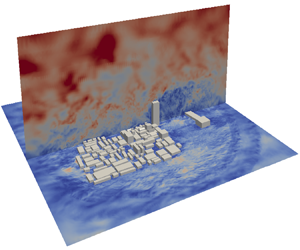
Figure 4 visualizes the overall flow field using contour plots of the instantaneous velocity magnitude on a vertical plane through the centre of the domain and on a horizontal plane at 1 m above ground level. The contour plots visualize the large-scale turbulence structures in the boundary layer as well as the complexity of the flow within the urban canopy.

Figure 4. Instantaneous contours of the velocity magnitude for a vertical plane at the centre of the domain and a horizontal plane at 1 m from the ground.
Figure 5 focuses on the flow in the test house, displaying contours of the time-averaged velocity and temperature fields on a vertical plane through the centre of the house for the daytime (top) and nighttime (bottom). The daytime case has a low mean indoor air velocity, which indicates that ventilation will mainly be due to turbulent air exchange. The nighttime case exhibits a more pronounced mean flow through the window, indicating a potentially higher ventilation rate. The differences between the daytime and nighttime velocity patterns are related to the differences in the temperature fields. During the day the roof is heated by solar radiation, thereby establishing a strong vertical temperature stratification. During the night the temperature is much more uniform throughout the indoor space.

Figure 5. Contour plots of the time-averaged velocity magnitude and temperature on a vertical plane through the centre of the house. Daytime case (left) shows a low mean velocity and thermal stratification; nighttime case (right) shows a clear mean flow pattern and more uniform temperature with height.
Figure 6 visualizes how these differences in the temperature distribution result in very different ventilation patterns by showing the time evolution of the scalar field on a vertical plane crossing both the window and skylight openings. During the daytime (top row), the stable temperature stratification results in a highly non-uniform ventilation of the indoor space, with the scalar concentration below the window opening much higher than the concentration near the ceiling. At night (bottom row), the more uniform temperature results in a more uniformly ventilated indoor space.

Figure 6. Time evolution of the scalar field after uniform initialization inside the house. Daytime case (top) shows non-uniform ventilation with height; nighttime case (bottom) shows higher flow rate and more uniform ventilation.
4.3 Validation of ACH predictions
As introduced in § 3.5, ventilation rates are calculated using both the scalar concentration decay method, and the velocity integration method. Figure 7 presents the resulting comparison between the field measurements and the LES predictions for both the daytime and nighttime cases. Considering the daytime case, the values obtained from the field measurement and the LES agree very well. The difference between both LES estimates is 16 %, with values of 8.41 and 9.90 hr $^{-1}$ for the scalar decay and the velocity integration methods, respectively. The experimental value is in between both estimates at 9.65 hr $^{-1}$. Despite the non-uniformity of the scalar field under daytime conditions, the scalar decay method provides a good estimate of the overall air exchange rate. This good agreement can be attributed to the central location at which the scalar decay was monitored; locations closer to the ceiling would over predict the ventilation rate, while closer to the ground an under prediction would be obtained. The velocity integration method reveals significant fluctuations over time, confirming the importance of unsteady, turbulent air exchange through the openings.

Figure 7. The ACH time series, mean value and standard deviation, estimated using the velocity integration method and the scalar concentration decay method for (a) daytime and (b) nighttime validation cases. Comparison with the mean and standard deviation of the ACH value obtained from the field measurement.
Considering the nighttime case, the difference between both predictions is slightly higher at 24 %, with values of 21.78 and 17.14 hr $^{-1}$ for the scalar decay and the velocity integration methods, respectively. The measurement produced a slightly lower value at 16.17 hr $^{-1}$. There are two likely explanations for these observed differences. First, even though the space is more uniformly ventilated during the night than during the day, the result of the concentration decay method can still be very sensitive to the location at which the scalar decay is monitored. Small differences in the internal flow pattern, such as a slight shift in the direction of the outdoor air stream coming in through the window can result in non-negligible variations in the decay rate (see figure 6). Second, the simulations do not account for infiltration through small gaps in the building envelope. Infiltration can lead to additional air exchange, and it can also decrease the pressure differences between the indoor and outdoor environment, which can further modify ventilation pattern.
The above comparison of the ventilation rates demonstrates the predictive capability of LES for combined wind- and buoyancy-driven ventilation in a complex urban environment. The LES predicts measured ventilation rates within 24 %, and the simulations reproduce the significant difference between daytime and nighttime ventilation rates. In the next section, we leverage the validated LES set-up to perform predictive simulations under different weather conditions and investigate whether flow similarity can be leveraged to efficiently characterize the ventilation in the home under a wide range of weather conditions.
5. Richardson number similarity for natural ventilation
This section first introduces ventilation Richardson number similarity for natural ventilation. Subsequently, results from two simulations that have the same ventilation Richardson number but different operating conditions in terms of the wind speed and indoor/outdoor temperature difference are compared to confirm their similarity. Finally, simulations for a range of ventilation Richardson number and wind directions are performed to establish a similarity relationship that can efficiently account for the variability in weather conditions.
5.1 Ventilation Richardson number,  $Ri_v$

Natural ventilation is driven by two driving forces, i.e. buoyancy and wind. Hence, the natural ventilation rate in a home will be a function of a large number of parameters affecting these two driving forces. For a fixed urban setting and natural ventilation opening configuration, one can expect the following dependency:
 \begin{equation} Q_{nv} = f(T_{in}, T_{out}, T_{roof}, T_{wall}, T_{floor}, U_{wind}, \theta_{wind}, H, g, A_{opening}), \end{equation}
where  $T_{in}$ and $T_{out}$ are the indoor and outdoor air temperatures, $T_{roof}$, $T_{wall}$ and $T_{floor}$ are the roof, wall and floor surface temperatures, $U_{wind}$ and $\theta _{wind}$ are wind speed and direction, $H$ is the height of the house, $g$ is the gravitational acceleration and $A_{opening}$ is the effective area of the natural ventilation openings. The inherent variability in these parameters, due to varying weather conditions and indoor heat gains, makes it challenging to design natural ventilation systems (Reference Boulard, Kittas, Roy and WangBoulard, Kittas, Roy, & Wang, 2002; Reference Jiang and ChenJiang & Chen, 2002; Reference Liu, Pan, Cao, Long, Jiang and ChenLiu et al., 2019; Reference Srebric, Vukovic, He and YangSrebric et al., 2008; Reference van Hooff and Blockenvan Hooff & Blocken, 2010).
As a first step towards reducing the dimensionality of the problem, we consider that, for a certain construction of a home, the different temperatures are likely to be correlated. This is demonstrated in figure 8, which shows scatter plots of hourly temperature measurements during daytime (red) and nighttime (blue) together with the best linear fit. The plots indicate that  $T_{out}$ is correlated with ${\rm \Delta} T = T_{out}-T_{in}$, $T_{roof}$, $T_{wall}$ and $T_{floor}$. Hence, for a given outdoor temperature, wind speed and wind direction, we can expect a single value for the ventilation rate in a specific house. This reduced dependency is generally reflected as follows in analytical or empirical envelope flow models (Reference De Gids and PhaffDe Gids & Phaff, 1982; (2017), CEN; Reference Hunt and LindenHunt & Linden, 1999; Reference Larsen and HeiselbergLarsen & Heiselberg, 2008; Reference WarrenWarren, 1978; Reference Warren and ParkinsWarren & Parkins, 1984):
 \begin{equation} Q_{nv} = f({\rm \Delta} T / T_{ref} \boldsymbol{\cdot} g \boldsymbol{\cdot} H, U_{wind}, \theta_{wind},A_{opening}). \end{equation}
Figure 8. Correlation between the measured temperatures (circles) and best linear fit (dashed lines) during daytime (red) and nighttime (blue).
To further reduce the dimensionality of the problem, we define the dimensionless natural ventilation flow rate, as well as the dimensionless ventilation Richardson number  $Ri_v$, which quantifies the ratio of the driving forces due to buoyancy and wind
 \begin{equation} Q'_{nv} = \frac{Q_{nv}}{A_{opening}\boldsymbol{\cdot} U_{wind}};\quad Ri_v = \frac{{\rm \Delta} T / T_{ref} \boldsymbol{\cdot} g \boldsymbol{\cdot} H }{ U_{wind}^2}. \end{equation}
The non-dimensional ventilation rate can then be written as a function of only two input parameters
 \begin{equation} Q'_{nv} = \phi(Ri_v, \theta_{wind}). \end{equation}
The main assumption in this similarity relationship is that, for a constant  $Ri_v$, small changes in the non-dimensional indoor temperature field, caused by the different correlations of the floor, wall and roof surface temperatures with ${\rm \Delta} T/T_{out}$, will have a limited effect on $Q'_{nv}$. This assumption will be verified in the following section, before identifying the functional form of $\phi$ in § 5.3.
5.2 Verification of the use of similarity relation
The  $Ri_v$ similarity proposed in § 5.1 is verified by performing simulations for two different ventilation configurations: daytime ventilation in the skylight/window configuration, and nighttime ventilation in the skylight/floor-level vent configuration. For each of these ventilation scenarios, two simulations with the same $Ri_v$ and $\theta _{wind}$, but different indoor–outdoor temperature differences ( ${\rm \Delta} T$) and reference wind speeds ( $U_{wind}$) are performed. For the reference case, the wind and outdoor temperature boundary conditions are based on the field measurements; the measured ${\rm \Delta} T$ and $T_{out}$ are used to determine the corresponding $Ri_v$. For the similar case, a different wind speed is selected, and the corresponding ${\rm \Delta} T$ is calculated such that the two new parameters result in the same $Ri_v$. The outdoor temperature ( $T_{out}$) and indoor surface temperature boundary conditions ( $T_{roof}$, $T_{wall}$ and $T_{floor}$) are obtained using the correlations between ${\rm \Delta} T$ and these wall surface temperatures, shown in figure 8. It is noted that ${\rm \Delta} T$, and hence the actual $Ri_v$, are ultimately outputs of the simulations, i.e. their actual values depend on the indoor temperature calculated by the simulation. For each simulation it was verified that the difference between the intended and actual $Ri_v$ was negligible.
Table 2 summarizes both the simulation settings and the results for the non-dimensional ventilation rates of the four cases. Figures 9(a) and 9(b) show the corresponding time series of dimensional and non-dimensional ventilation rates as well as their frequency distribution. The dimensional ACH values differ significantly, but after non-dimensionalizing the time series and distributions collapse. The difference between the mean non-dimensional ventilation rates for the similar cases is 6.5 % for the daytime skylight/window configuration and 3.6 % for the nighttime skylight/floor-level vent configuration. These small differences are likely due to differences in the non-dimensional indoor surface temperature boundary conditions between the cases. These differences can have a secondary effect on the ventilation pattern and resulting non-dimensional flow rate; this effect is not represented in the proposed similarity relationship. However, the cost benefit of significantly reducing the parameter space warrants introducing this relatively small (<10 %) uncertainty in the results.
Table 2. Summary of operating conditions ( $Ri_v$, $\theta _{wind}$, $U_{wind}$ and ${\rm \Delta} T$) and simulation results for the verification of Richardson number similarity. Bold has been used in the table to emphasise how the time series for the non-dimensional ventilation rate and its distributions collapse while the Richardson numbers have stayed the same.


Figure 9. Time series (top) and its frequency distribution (bottom) of ACH (left) and non-dimensional ventilation rate (right) for the (a) daytime and (b) nighttime verification cases, demonstrating the validity of the proposed  $Ri_v$ similarity.
5.3 Functional form and validation of the similarity relationship
In this section, the functional form of the similarity relationship is established and tested. First, the value of  $Ri_v$ is varied with $\theta _{wind}$ fixed to the dominant wind direction; second, the combined effect of $Ri_v$ and $\theta _{wind}$ is determined; third, the ventilation rates obtained from the similarity relationship are compared withthe available field measurements.
5.3.1 Effect of $Ri_v$ with fixed $\theta _{wind}$


The impact of  $Ri_v$ on the non-dimensional ventilation rate $Q'_{nv}$ is investigated by performing simulations for a fixed wind direction of 330 $^\circ$, which was the dominant wind direction in the slum neighbourhood during the field campaign. For the nighttime conditions, we perform simulations with $Ri_v=[-0.85, -0.6, -0.4, -0.2, -0.0]$, while for the daytime, we consider $Ri_v=[+0.0, +0.2, +0.4, +0.6]$. The difference between the nighttime and daytime cases is that the temperature boundary conditions are defined differently, using the respective correlations obtained from the measurement data presented in figure 8.
Figure 10 presents the results, plotting  $Q'_{nv}$ as a function of $Ri_v$ for $\theta _{wind}=330^\circ$. The plot represents the mean and standard deviation of the non-dimensional ventilation rate time series predicted by the LES. The two different colours correspond to the daytime cases with indoor thermal stratification (red) and to the nighttime cases with a uniform indoor temperature (blue). The case with $Ri_v = 0.0$ is simulated for both daytime and nighttime conditions, and the small difference between these results confirms that changes in the floor and ceiling temperatures have a limited effect on $Q'_{nv}$. Overall, the ventilation rate is lower during daytime than nighttime, primarily due to the different temperature distributions. During the day, the indoor environment is stably stratified, and the neutral line, where the indoor and outdoor temperatures are equal, is close to the roof. This limits buoyancy-driven ventilation, which is reflected in the relatively slow increase of $Q'_{nv}$ with $Ri_v$. During the night, the more neutral stratification of the indoor environment in combination with the negative temperature difference ${\rm \Delta} T$, supports buoyancy-driven ventilation, resulting in more significant increases in $Q'_{nv}$ as $Ri_v$ becomes more negative.

Figure 10. Non-dimensional ventilation rate as a function of ventilation Richardson number for a fixed wind direction of 330 $^\circ$.
Although the daytime and nighttime scenarios show a different slope, both cases exhibit roughly linear increases in  $Q'_{nv}$ as the absolute value of $Ri_v$ increases over the range of $Ri_v$ considered. It is reasonable to assume that a similar linear dependency will hold for the other wind directions; hence, the following section will consider different wind directions, but only simulating two points for each scenario: $Ri_v$= $-$0.85, $-$0.00 for nighttime, and $Ri_v= +0.00$, 0.60 for daytime.
5.3.2 Combined effect of $Ri_v$ and $\theta _{wind}$


For wind engineering applications, it is standard practice to explore all wind directions with a 10 $^\circ$ resolution. In the context of assessing natural ventilation, there is an opportunity to reduce the number of required simulations by considering the prevalence of the different wind directions at the location of interest. Figure 11(a) shows the polar histogram of the wind direction data, indicating that the wind is predominantly coming from the north-west. This polar histogram was divided into eight sectors with an equal probability of occurrence, resulting in a minimum resolution of about 10 $^\circ$ around the most dominant wind direction. The median wind directions of these sectors were selected to perform the simulations with the four different values for $Ri_v$. This process supports accurate estimates of the natural ventilation flow rates for the most prevalent wind directions, while accepting an increased uncertainty in the estimates for wind directions that rarely occur.

Figure 11. (a) Polar histogram of wind direction data to determine the eight wind directions to be simulated; (b) perspective view of the neighbourhood buildings indicating the selected wind directions.
The non-dimensional ventilation rates  $Q'_{nv}$ obtained from the 32 LES simulations with varying $\theta _{wind}$ and $Ri_v$ are plotted in figure 12. A striking observation is the small influence of $\theta _{wind}$ compared with the influence $Ri_v$. The maximum variation in $Q'_{nv}$ due to a $\theta _{wind}$ change, observed for $Ri_v=-0.85$, is only approximately 8 %. In contrast, the increase in $Q'_{nv}$ from $Ri_v=0.00$ to $Ri_v=-0.85$, averaged over all wind directions, is 270 %.

Figure 12. Surrogate response surface for non-dimensional ventilation rate with respect to  $Ri_v$ and $\theta _{wind}$.
The unexpectedly small impact of the wind direction can be tied back to the flow pattern around the test house. The movies in the supplementary materials available at https://doi.org/10.1017/flo.2023.4 present the instantaneous velocity fields within a 15 m radius from the test house for all eight wind directions and  $Ri_v=-0.00$ at a height of 3 and 1 m. The velocity field at 3 m height, which is slightly above the average building height, is significantly affected by the incoming wind direction. Buildings that exceed this height are more sparsely distributed, such that the stagnation regions and wake patterns around these buildings change significantly with varying wind directions. However, the flow field at 1 m height, which is below the test house roof height, is not significantly different when the wind direction changes. This is especially pronounced for the flow in the courtyard where the window opening is located. These results indicate that in densely packed urban areas, the airflow between buildings is strongly determined by the layout of the urban canopy and the impact of the wind direction can be significantly reduced.
5.4 Validation of the similarity relationship
The accuracy of the similarity relationship developed in § 5.3.2 is evaluated in figure 13(a), considering the 4 measurements in the skylight/window configuration. The figure shows a scatter plot of the ACH values obtained by the surrogate model, evaluated at the  $Ri_v$ and $\theta _{wind}$ observed during the measurements, vs the measured ACH values. For the nighttime cases (blue/skyblue), the discrepancies between the predicted ACH value and the mean value from the measurement is less than 9 %. Figure 13(b) shows that, during these measurements, the surface temperatures corresponded closely to the values obtained from the correlations used to define the boundary conditions in the LES. For the daytime cases, the discrepancies are slightly higher, with the surrogate model over predicting the measurements by 37 %. This discrepancy is higher than expected based on the validation presented in § 4. Figure 13(b) shows that a likely explanation is that the roof temperature recorded during these measurements was approximately 3.26 $^\circ$C lower than the temperature obtained from the correlation used to define the roof temperatures in the LES that informed the surrogate model. As such, the indoor environment was less stratified during these experiments than what would be expected on average based on the correlations, which reduces the ventilation rate. The surrogate model can be expected to be more accurate when considering the average ventilation rate that the home will see over a longer time period, since the correlations represent the average condition.

Figure 13. (a) Validation of the surrogate model using  $Ri_v$ similarity for the skylight/window configuration; (b) correlation between the different temperature measurements, highlighting the values during the skylight/window ventilation experiments. Daytime cases are shown in red, nighttime cases are shown in blue.
In a final step, we explore whether the surrogate model can predict ventilation in the home more generally, considering all four opening configurations for which experiments were performed (see figure 1(b). The aim of this analysis is to provide initial insight into the importance of the specific opening locations in the home. Figure 14 presents the comparison of the surrogate model predictions against all 17 measurements under the four different configurations. The model correctly captures the trend in the measurements, with an average discrepancy of 27 %. This result indicates that in this dense urban setting the opening locations are also secondary effects.

Figure 14. Validation of the surrogate model using  $Ri_v$ similarity for all ventilation configurations.
6. Conclusion and future work
This paper has proposed and validated an efficient strategy for using CFD to predict natural ventilation flow rates in a specific house as a function of highly variable boundary conditions. First, urban-scale LESs were shown to predict field measurements of the ventilation rate in a single-room urban slum home with a window and a skylight within 25 %. Next, 32 simulations were used to establish a similarity relationship that expresses the dimensionless ventilation rate as a function of just two parameters: the dimensionless ventilation Richardson number and the wind direction. The main assumption in this similarity relationship, namely that for a constant ventilation Richardson number small changes in the non-dimensional indoor temperature field will have a limited effect (<10 %) on the dimensionless ventilation rate, was verified to be correct. The resulting surrogate model indicates a strong dependency of the non-dimensional ventilation rate on the ventilation Richardson number, while the wind direction only has a small secondary effect. The limited effect of the wind direction is attributed to the density of the urban canopy below the roof height of the test building. Comparison of the surrogate model predictions with four different field measurements in the configuration with the window and the skylight open reveals differences ranging from 9 % to 37 %. The higher discrepancies occur when the roof surface temperature is lower than average during the field measurements, since the similarity relationship was designed to represent the average conditions.
In summary, this paper has shown that LESs can efficiently inform accurate, building-specific similarity relationships for natural ventilation flow rates. In future work, we will explore the use of a building thermal model to (i) define the correlations for the surface temperature boundary conditions in the absence of field measurements, and (ii) obtain predictions of the seasonal and yearly distributions of the ventilation rate. Furthermore, we will investigate how the density of the urban canopy, as well as the specific building configuration and location change the influence of the wind direction on the ventilation rate. The proposed modelling strategy has the potential to support performance-based design of natural ventilation systems to improve occupant health and well-being.
Supplementary movies
Supplementary material and movies are available at https://doi.org/10.1017/flo.2023.4. Raw data are available from the corresponding author (Y.H.).
Acknowledgements
The authors gratefully acknowledge the contributions of their collaborators S. Luby, L. Kwong and the research team at icddr,b in Bangladesh. The research meets all ethical guidelines, including adherence to the legal requirements of the study country.
Funding statement
This research was funded by a seed grant from the Stanford Woods Institute Environmental Venture Projects program and supported by the Stanford Center at the Incheon Global Campus (SCIGC) funded by the Ministry of Trade, Industry, and Energy of the Republic of Korea and managed by the Incheon Free Economic Zone Authority. The simulations were performed using the Extreme Science and Engineering Discovery Environment (XSEDE), which is supported by National Science Foundation grant number CI-1548562.
Declaration of interests
The authors declare no conflict of interest.
Author contributions
Y.H. designed and conducted experiments, performed simulations and formal analysis of results and wrote the original draft of the manuscript. C.G. created the research plan, supervised the project, and reviewed and revised the manuscript.


 Open access