Introduction
Shape grammars provide a formal mechanism to support design space exploration using visual replacement rules (Stiny, Reference Stiny1980). This formalism is defined with an initial shape and a set of visual rules. Depending on the domain of the computation, a particular algebra and its supported operations are applied to transform the given initial shape (Stiny, Reference Stiny2006).
A visual rule is represented in A → B form, where A stands for the left-hand side (LHS) shape of the visual rule and B is the right-hand side shape (RHS). Assume that S is the initial shape, application of this rule to the initial shape is performed in three steps: (1) a Euclidean transformation of the LHS shape, that is Τ(A), is computed such that it is embedded in S: T(A) ≤ S; (2) the embedded part is subtracted from the initial shape, that is, S−Τ(A); (3) the same transformation is applied to B, that is, Τ(B), and added to the modified S, that is, S−Τ(A) + Τ(B). As a result, a given initial shape is modified according to the embedding relation of the LHS shape with the initial shape using a well-defined replacement operation. Although the formalism defines a simple way to transform a given shape, its representational power can be used to generate different designs in a particular style with a properly defined shape grammar (Stiny & Mitchell, Reference Stiny and Mitchell1978; Flemming, Reference Flemming1987; Pugliese & Cagan, Reference Pugliese and Cagan2002; McCormack et al., Reference McCormack, Cagan and Vogel2004).
Ever since the shape grammar formalism is introduced, a considerable effort is put on the computational modeling of shape grammar interpreters. The challenge is on the difficulty of automatic computation of embedding emergent parts. When visual rules transform a given shape with rule applications, shapes split, and fuse to form new patterns. Such productions may generate new forms and provide new embedding possibilities that emerge only after rule applications. A designer, who uses a computer-based solution, would like to be able to reinterpret these parts since they become visible to them. Therefore, the representations of the resultant shapes in computers should be adaptive to new interpretations and conform the needs of a designer who continuously exploits the ambiguity in resultant forms.
In this research, we propose a novel approach to solve the part embedding problem. The proposed approach implements an optimization algorithm to compute the embedded parts using weighted representations of the initial shapes, in a fast and accurate way; we developed a particle swarm optimization-based solution. Inspired by our preliminary work (Keles, Reference Keles2015), we designed and implemented a parallel algorithm that runs on thousands of hardware threads on a graphics processing unit (GPU) simultaneously to compute embeddings. The motivation behind this research is to solve two primary problems of the optimization-based part embedding methods: (1) stucking into local minima and (2) high execution time. We also aim to provide many different embedding alternatives to the designer simultaneously so that the designer can explore the design space more effectively by selecting the desired embedding to apply the rule. We believe that the improvement in the embedding accuracy and the response time, together with many different embedding options, support the designer's cognitive processes better.
In this paper, we explain our solution in detail both with respect to its design and implementation. The paper is organized as follows. In the next sub-section, we introduce the particle swarm optimization algorithm in its general form. Following that, we provide a brief introduction to the general purpose programming on GPUs. After these introductory sections, we discuss the current state of the art in the section “Related works”. In the section “The PSO approach for part embedding problem”, we explain our particle swarm optimization (PSO)-based solution, particularly for sub-shape embedding problem. Following that, in the section “GPU–PSO-based part embedding approach”, we discuss our GPU-based solution. In the section “Results and discussion”, we provide a set of results and discuss the impact of our approach. Then, we finalize the paper with a brief conclusion at the end.
The PSO algorithm
PSO is a population-based iterative algorithm, which optimizes a problem using a method that is inspired by the movements of a flock of birds or schooling of fishes. The algorithm is based on the movement of individuals in a population in the direction considering a combination of the population's best fitness value and its own best fitness value. It is invented by Russell Eberhart and James Kennedy in 1995 and has been used in many optimization problems since then (Poli, Reference Poli2008).
In evolutionary terms, a population is called a swarm, and an individual is called a particle. A fitness function is defined according to the problem and – similar to evolutionary approaches – is designed to generate a score (i.e., a real value) using a set of optimization parameter values as its inputs.
In a PSO formulation, a number of particles (i.e., candidate solutions) search over the problem domain by interacting with their environment and with other particles in the swarm to improve their fitness. Each particle in a swarm has two main attributes; velocity and position. The position of a particle corresponds to a specific solution to the problem, while velocity is used to determine the direction of the particle in the next iteration. Hence, during the iterations, two reference values guide the movement of a particle: (1) best fitness value achieved by the particle so far and (2) best fitness value of the swarm recorded so far. Each particle has a memory to keep their best fitness value and corresponding position (i.e., the solution parameters) at a particular time during the searches. Moreover, the swarm has a memory that keeps the best fitness value of all particles obtained so far and the corresponding position. The next position of a particle i is determined using the two simple formulae given below:
 $$\eqalign{\vec {v}_i^{\,t + 1} & = \vec {v}_i^{\,t} + A_{\rm L}\,{\ast}\,\hbox{rand}(0\comma \,1)\,{\ast}\,({\overrightarrow {bx_i^t}} - \vec {x\;}_i^t ) \cr & \quad + A_G\,{\ast}\,\hbox{rand}(0\comma \,1)\,{\ast}\,(\overrightarrow {gbx ^t} - \vec {x\;}_i^t )}$$
 $$\vec {x\;}_i^{t + 1} = \vec {x\;}_i^t + \vec {v\;}_i^{t + 1} $$
 In Eqs. (1) and (2): t represents discrete time steps,  ${\vec {v\;}}_i^t $ is the velocity of particle i at time step t, $\vec {x\;}_i^t $ is the position vector of the ith particle (i.e., current solution) at time step t, $\overrightarrow{{bx}^{t}_i} $ is the best position vector of the ith particle up to time step t, and $\overrightarrow {gbx^t}$ is the best position of the all particles obtained up to time step t.
In (1), A L and A G are the local and global acceleration constants, respectively. In this work, we set both of them to 1, hence balanced the contribution of the swarm and the particle. Assuming that we work in a d-dimensional search space, each dimension corresponds to a particular optimization parameter of the problem domain. In this domain,  $\vec {v}_{\rm i}$ is a d-dimensional velocity for the particle i and $\vec {x}_i$ is a d-dimensional position vector that contains the estimated values of the optimization parameters.
PSO is initialized with a set of particles with random positions and each particle searches for some optima by updating its velocity and position for a number of generations. In (1), the velocity direction is computed using a random number generator, that is, rand(0,1) function that produces values that are driven from a uniform distribution in the range (0, 1). This stochastic nature helps efficient spatial exploration. The stopping condition is set either with a constraining iteration number or with a minimum error criterion.
In the proposed solution, the vector  $\vec {x}_i$ represents the transformation parameters of the LHS shape such that $T_{{\vec {x}}_i}(A)$ embeds the shape A in the initial shape S, that is, $T_{{\vec {x}}_i}(A) \le S$. Here, the subscript i represents a candidate solution determined by the particle i in the swarm. Therefore, the swarm in a particular region of the initial shape, S, collaborates to decide the best embedding in that region that satisfies a given tolerance constraint.
General-purpose computing on graphics processing units (GPGPU) using CUDA
Today, GPUs are not only used for graphical computations but are also used for general purpose computations that require high performance with their many-core architectures. The release of CUDA by NVidia in November 2006 enabled utilization of graphics processing units for general purpose computations in a more suitable way by providing a programming model that enables utilization of data parallelism through the abstractions for thread groups, shared memory, and thread synchronization (Owens et al., Reference Owens, Houston, Luebke, Green, Stone and Phillips2008). For this purpose, it is defined as a set of extensions to C programming language. In order to utilize this high computational power, a serial algorithm needs to be redesigned both with respect to its computational flow and data access patterns.
Modern GPUs are composed of an array of streaming multiprocessors (SMs) that are composed of many parallel executing hardware threads that execute a given sequential GPU program, which is called as a kernel, in parallel. The scheduling and management of these threads are made by SMs using a single instruction multiple thread (SIMT) architecture. So, each thread in an SM executes the same instruction at a particular time while executing a given kernel.
The CUDA programming model enables utilization of this architecture by instantiating executions of the codes written as sequential programs for one thread on many hardware threads in an SM of GPU, simultaneously. Hence, it is a scalable parallel programming model. In this model, every kernel is defined to solve a particular computational problem for one thread; yet each thread actually solves only a part of the problem. A given problem is solved by executing many blocks of concurrently executing threads.
A template utilization of CUDA programming model can be summarized as follows: (1) allocate necessary memory space on the device, that is, the GPU global memory; (2) copy the necessary data that need to be operated on to the GPU memory; (3) launch the GPU kernel(s); and (4) copy the computed results, that is, modified data, back to the CPU memory.
We provide a detailed discussion about our GPU-based PSO solution in the section “GPU–PSO-based part embedding approach”.
Related work
Since the seminal work of Stiny and Gips on shape grammars (Stiny & Gips, Reference Stiny and Gips1972), many researchers have focused on computational solutions that support shape grammar formalism. The crucial part of such a solution is the ability to support embedding emergent shapes during the generation process.
Earlier solutions to the embedding problem are primarily based on Krishnamurti's maximal element-based representation (Krishnamurti, Reference Krishnamurti1980, Reference Krishnamurti1981; Krishnamurti & Giraud, Reference Krishnamurti and Giraud1986; Chase, Reference Chase1989; Krishnamurti, Reference Krishnamurti1992; Tapia, Reference Tapia1999; Chau et al., Reference Chau, Chen, McKay and Pennington2004; Jowers, Reference Jowers2006; McCormack & Cagan, Reference McCormack and Cagan2006; Jowers & Earl, Reference Jowers and Earl2010). Most of these approaches detect emergent parts by representing shapes with some presumed analytical or geometric abstractions, that is, straight lines, parametric curves, rectilinear shapes, etc. The maximal representation is primarily based on the representation of shape parts as parts of some maximal elements. These maximal elements are called as carriers. The parts on these carriers are represented with their boundaries. For efficient part searches, the parts on the same carriers are sorted according to their boundaries and utilized as a list. Tapia (Reference Tapia1999) developed one of the best implementations of this idea, with a graphical user interface (GUI) that works with rectilinear shapes.
In addition to the researches that solve the embedding problem with straight lines and rectilinear shapes, some approaches propose solutions for the curved shapes. Chau et al. (Reference Chau, Chen, McKay and Pennington2004) employed a similar method to the maximal element-based approaches to implement embedding shapes with circular arcs. Circular arcs share similar embedding properties with the straight line segments in their parametric representations; hence, their work adapts maximal representation of lines to circular arcs. McCormack and Cagan (Reference McCormack and Cagan2006) provided a parametric sub-shape recognition solution that decomposes shapes into a hierarchy of sub-shapes ordered by their decreasing restrictions. They represent the curved shapes with their underlying straight line representations (i.e., structure). Hence, matching is performed in two stages; first, the straight line representations of the shapes are matched, and then a validation is performed that matches curved parts.
Jowers extended the embedding approach for straight line elements to work with free-form curves (Jowers, Reference Jowers2006). His representation defines shape elements using their carriers, boundaries, and the types of curves. According to this solution, binary shape operations can be performed only if the two shape elements are of the same type and only if they lie on the same carrier. Jowers and Earl (Reference Jowers and Earl2010) then extended this approach to a more generic form for curved shapes such that, shapes need not be represented with distinct points and parts, but are compared using their intrinsic properties of their parametric curve segments, that is, the curvature. They used differential geometry to compare parametric curve segments, where the intrinsic properties of curvature are defined with respect to the curve arclength. They defined a formal representation to compare curved shapes according to the types of the constituent curve segments. However, such a representation may provide a limitation on the generic nature of emergent part detection in a way similar to the representations of shapes using a set of predefined shape primitives.
Shape grammar formalism provides necessary algebras and Boolean operations defined in these algebras to perform visual computation with shapes, regardless of their representation and creation history of their constituent parts. This is the challenge that needs to be taken by the approaches that solve the emergent part detection problem. Although analytical approaches provide solutions for different types of shapes, there are two primary computational problems in practice while working with drawings/sketches: (1) we need to know the analytical forms of constituting parts of shapes before operating, and (2) we need to compute the parameters of the analytical forms from drawings accurately. Knowing the first one does not make the computational problem of parameter estimation easy, especially in a system where a shape constantly changes using different shape rules. These challenges push the practical solutions to define some restrictions on the types of shapes that a shape grammar implementation supports, that is, working only with rectilinear shapes. Hence, a generic solution needs to treat shapes indifferently from the parametric types of their constituent parts.
Recently, new approaches have been proposed as a result of this need and provide alternative solutions to the emergent sub-shape detection problem by considering shapes as continuous entities. In these approaches, shapes are treated as they are and unlike the previous approaches, assumptions on the analytic forms of shapes are avoided. Although each one uses different representations for shapes and different approaches for part embeddings, they all treat shapes that contain straight lines, circular arcs, or free-form curves or all, equally such that the shape representations become invariant to constituting analytical forms. They either use some registration points as vertices to shape graphs to resolve structure and perform part matchings for graph edges (Keles et al., Reference Keles, Ozkar and Tarı2010; Grasl & Economou, Reference Grasl and Economou2013); use pixel-based representation and image processing algorithms (Jowers et al., Reference Jowers, Hogg, McKay, Chau and Pennington2010); use weighted representation of shapes and evolutionary optimization algorithms (Keles et al., Reference Keles, Ozkar and Tarı2012; Keles, Reference Keles2015). In all these approaches, shapes are not treated as a composition of a set of pre-defined analytical forms but treated as continuous entities.
Keles et al. (Reference Keles, Ozkar and Tarı2010) represented shapes using over-complete graphs and determined part embeddings using the attributes of the graph nodes which define the geometric relations among the nodes in the spatial domain. Another graph-based solution is proposed by Grasl and Economou (Reference Grasl and Economou2013) that supports emergent shape detection and parametric rule applications. They perform parametric part matchings by defining restrictions on shape topologies. Both approaches need to modify the corresponding graphs when a rule application modifies a shape. This is the main disadvantage of using graph-based representations. The difficulty is on this dual interpretation and switching back and forth between the shape and its representational form.
Jowers et al. (Reference Jowers, Hogg, McKay, Chau and Pennington2010) provide an image-based solution to the emergent part detection problem where image pixels are treated as points in two-dimensional (2D) space and the Houssdorff distance is used as a metric to define part embeddings. They need to define manual thresholds to accept embeddings according to the given shapes.
Keles et al. (Reference Keles, Ozkar and Tarı2012) proposed a solution that considers the part embedding problem as an optimization problem using weighted representations of given shapes. Shapes are transformed to a weighted domain using a partial differential equation-based diffusion function. The optimization in this domain is implemented with a genetic algorithm. The cost function in the proposed implementation is defined as the sum of the squared distances between a part of an initial shape and the rule shape.
The two primary disadvantages of using an optimization-based method are the convergence time and local minima problem. In order to solve both problems, Keles (Reference Keles2015) proposed a parallel genetic algorithm-based implementation of the embedding problem using multiple CPU cores simultaneously. Being the preliminary work of this research, Keles (Reference Keles2015) depicted that running multiple sub-populations concurrently in the search space not only optimizes the execution time, but also reduces the probability of getting stuck in local minima, that is, an undesired solution, considerably. We improved that work by changing the utilized optimization algorithm, since determining the selected evolutionary parameters in a genetic algorithm, that is, mutation rate, cross-over rate, Elite count, etc. is more complicated.
There are other evolutionary approaches that are utilized with shape grammars (Ang et al., Reference Ang, Chau, Mckay and de Pennington2006; Lee & Tang, Reference Lee and Tang2009; O'Neil et al., Reference O'Neill, McDermott, Swafford, Byrne, Hemberg, Brabazon, Shotton, McNally and Hemberg2010); however, these approaches focus on solving the discovery of visual rule sequences to obtain a particular design with a given grammar. The evolution of the derivation, which is the product itself, is evaluated with a cost function to assess its usefulness. Determining the sequence of rules that generates a feasible production is out of the scope of this study.
In this work, inspired by the results of our preliminary work, we designed and implemented a massively parallel optimization solution to the part embedding problem. For optimization, we adapted a PSO-based method to minimize the same cost function that we used in Keles (Reference Keles2015). As in Keles (Reference Keles2015), this work also provides multiple simultaneous embeddings in the shape generation process, if desired. Moreover, simultaneous evaluation of the multiple results and selection of the best of best results among different sub-populations help locating the global solution. The contribution of this work to the existing literature is twofold: (1) adaptation of the particle swarm optimization algorithm in part embedding problem is studied for the first time and (2) implementation of a parallel PSO-based solution on GPU architectures in this problem domain is studied for the first time.
The PSO approach for part embedding problem
In this section, we discuss the fitness function and our data representation that we use in our optimization method. We also provide pseudocodes for our PSO-based part embedding solution.
In our implementation, the initial shape in a shape rule is represented as an image and a smoothed distance field is generated from this image using an exponential form of the standard distance function that we specified in our preliminary work (Keles, Reference Keles2015). On the other hand, the rule shapes are represented as images. Hence, the U 12 representation of the LHS shape is aligned with the W 22 representation of the initial shape. In the W 22 representation of the initial shape, the weights are zero on the shape pixels and they increase exponentially away from them. When an LHS rule shape is searched within the boundaries of this weighted representation, each candidate alignment of the LHS shape via different transformations produces a cost value that represents the total distance of the alignment to the initial shape. In a successful embedding scenario, an LHS shape is perfectly aligned with a part of the initial shape. In this case, the sum of the distance values corresponding to the alignment pixels of the distance field is almost zero. This is the cost of the alignment and we want to minimize this cost in order to optimize our search parameters. Therefore, our fitness function is actually the inverse of the cost function.
In our computational framework, an LHS shape is initially placed at the center of the initial shape. We then consider candidate similarity transformations of the LHS shape in the initial shape's local coordinates while embedding it to a part of the initial shape. Therefore, we search for four parameters: (1) scale(s), (2) rotation angle (θ), (3) translation on the x-axis (T x), and (4) translation on the y-axis (T y). Transformation of an LHS shape in the discrete domain corresponds to computing the transformed positions of each pixel in the shape. For this purpose, the following transformation matrix is utilized.
 $$\left[ {\matrix{ {s\,{\ast}\,\hbox{cos}(\theta )} & { - s\,{\ast}\,\hbox{sin}(\theta )} & {T_x} \cr {s\,{\ast}\,\hbox{sin}(\theta )} & {s\,{\ast}\,\hbox{cos}(\theta )} & {T_y} \cr 0 & 0 & 1 \cr}} \right].$$
When the pixel positions of an LHS shape are represented in homogeneous coordinates in column major order, multiplication of the matrix given in (3) with these coordinates generates the corresponding coordinates of the transformed LHS shape. These transformed coordinates are utilized to compute the cost of this alignment on the distance field that is generated from the initial shape. All the distance values that correspond to the transformed coordinates are accumulated to compute the total alignment cost. The PSO system is designed to optimize these four transformations parameters; namely the scale, rotation angle, and two translations. Hence, the search space is 4D. The pseudocode of our embedding PSO system is given below.As it is seen from the pseudocode given in Listing 1, it is a simple algorithm that can be implemented easily when the cost function is defined properly. We defined the cost function as in our previous work, which is proved to be effective in this domain (Keles, Reference Keles2015).
Although the implementation is easy when the number of particles in a swarm is increased, that is, to more than 50, computation of the cost function for a candidate takes a considerable amount of time and makes utilization of this method impractical for designers. In order to solve this problem, we designed a GPU-based solution to part embeddings.
Listing 1. Pseudocode of the PSO-based embedding algorithm

GPU–PSO-based part embedding approach
Given an initial image, we want a crowded swarm that is uniformly distributed over the image plane to explore the search space for part embeddings. However, when we increase the number of particles all around the image, computation of the fitness function takes a considerable amount of time, which makes this method unattractive for the users. Therefore, we designed a search space that allows simultaneous parallel executions of multiple swarms effectively.
The proposed approach is based on the partitioning of the image space into regular grids so that a number of swarms can work independently on different parts of the image plane. We can realize this by efficiently using parallel hardware threads in the GPU architecture. Then the resultant solutions, which come simultaneously from different parts of the image domain, can be evaluated on the CPU side.
For this purpose, we divide the image space in x- and y-directions into a set of non-overlapping tiles; and assign a number of GPU threads to work as particles in each tile (Fig. 1).
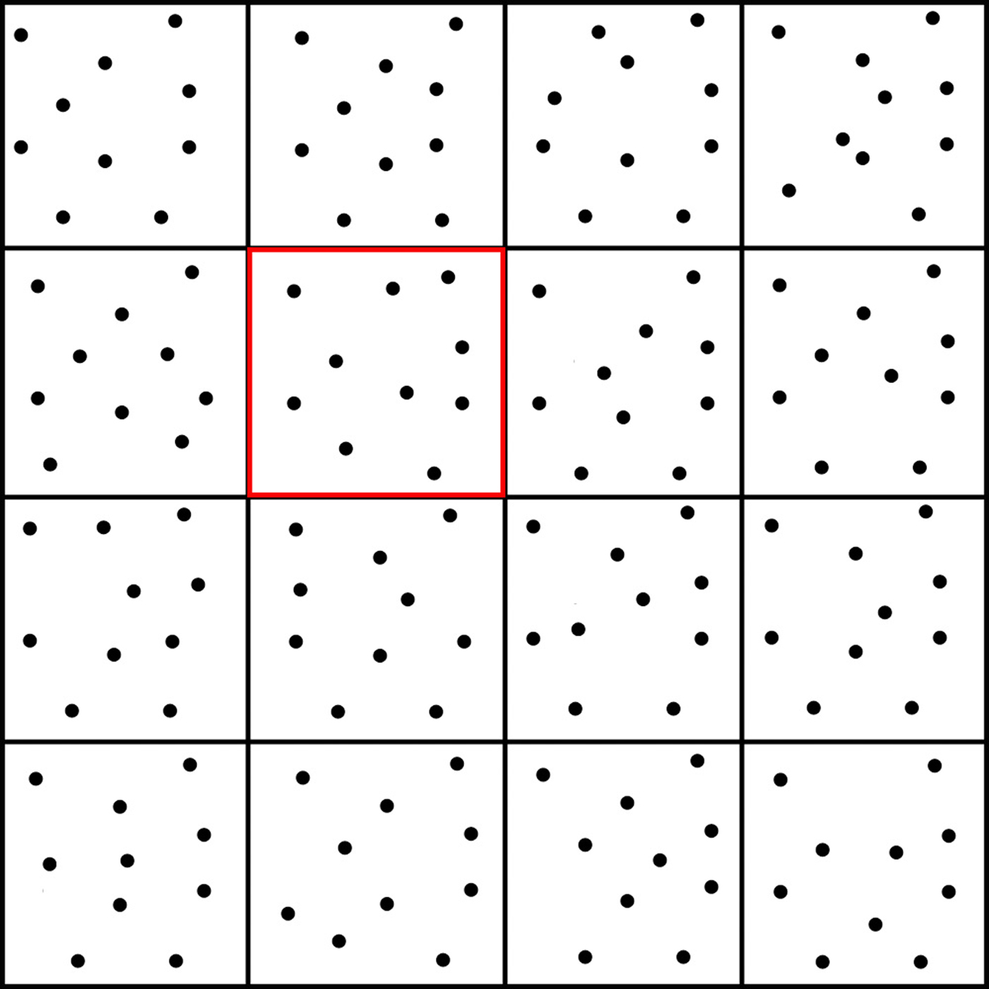
Fig. 1. Partitioning of the image space into a set of tiles is depicted. The points randomly assigned to each tile represent particles in the swarm.
In our solution, we consider all the threads in a tile as a swarm. Each swarm searches the corresponding image region within the tile boundaries. Hence, our approach considers the embedding problem as a multi-swarm optimization problem. The best solution in each tile can be compared with the other tiles to determine a global best solution; alternatively, each of these best solutions may be utilized to accept for simultaneous multiple embeddings. This depends on the user preferences; yet the solution is flexible enough to serve for both options. In addition, multiple-swarm design helps the approach to locate the global minimum almost all the time efficiently, due to the particles’ dense and uniform distribution in each tile. This reduces the probability of skipping a region in searches, which is the main cause of stucking in local optima in optimization-based algorithms.
GPU–PSO design
Except for the initialization of the position (X) and velocity (V) parameters, the entire embedding operation takes place on the GPU part using four CUDA kernels. Similar to the given pseudocode of the PSO algorithm (Listing 1), X i’s are initialized randomly, considering the parameter constraints, for each tile. In the default implementation, we only impose a translation constraint on X i’s parameters. The boundary coordinates of each tile are computed depending on the number of preferred sub-divisions and hence particles’ spatial movements are restricted within these coordinates. The user can also define desired scale constraints during the searches. During the PSO iterations on a GPU, these constraints are constantly checked for position updates and satisfied by clamping the values when they exceed the defined limits. In the following iterations, velocity and position updates regulate the behavior of such particles towards the inner parts of the tile. After the initialization, all the parameters are copied from CPU memory to device memory, that is, GPU memory.
We also need to copy the weighted representation of the initial shape to the device memory. As we stated in the section “The PSO approach for part embedding problem”, we need this representation to compute the fitness values for candidate solutions. The pre-computed distance field can be considered as an image as well. We copy this image to the device texture memory. The advantage of using texture memory is that texture memory is cached on-chip and these caches are optimized for memory access patterns that depict spatial locality. This is the case in the part embedding problem. When we compute a transformation, the accessed parts of the texture will be in close proximity to each other, considering the LHS shape as a whole, composed usually of connected pixel groups.
As it is shown in the flowchart in Figure 2, we implemented four kernel functions for GPU–PSO computations. For a predefined number of iterations, the four kernels are launched one by one. Note that the Evaluate Fitness kernel may be called multiple times in a sequence depending on the number of pixels in the LHS shape. Before explaining the kernels in detail let us define some parameters so that the kernels can be understood easily. Assume that we partitioned the initial shape into N tiles, hence we define N blocks, and each tile is assigned to T particles, hence we create T number of threads. The value of N depends on the preferred partitioning of the image tile, that is, parametric, hence can be changed by the user using the GUI. For example, for the partitioning shown in Figure 1, N is 16. We set the number of particles, T, in our experiments to 1024. Note that, the total number of particles searching the image space is N × 1024. This value is intentionally kept very high to assess the time performance of GPU–PSO implementation for the worst-case scenario where a lot of particles are utilized.
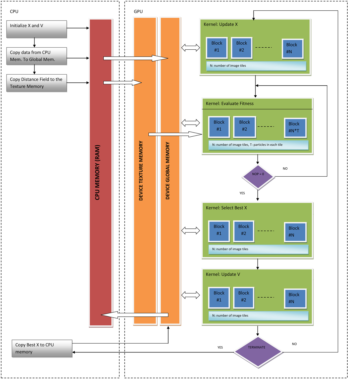
Fig. 2. Flowchart of the GPU–PSO-based embedding implementation. Data flow is also depicted on the same chart.
The implementation of CUDA kernels
In this section, we provide the pseudocodes of the CUDA Kernels and explain their design issues. During the execution of the GPU–PSO algorithm, the data are kept in the device memory all the time, and kernels are called one by one for a number of iterations.
GPU kernel, update X (Listing 2)
This is a small kernel, which reads X, V, and Constraints vectors and updates X using Eq. (2).
Listing 2. Pseudocode of the GPU kernel: update X in CUDA
GPU kernel, evaluate fitness (Listing 3)
Evaluation of the fitness of a particle requires: (1) transformation of the LHS shape pixels to the initial shape's local coordinates, (2) accumulation of the distance values using these transformed coordinates from the distance field, which is stored in the device texture memory. We need to compute this kernel for each and every particle in the population, that is, N × T particles. Therefore, this kernel is called for N × T number of blocks, each of which is actually computing the alignment cost of a particular particle. We used 1024 threads; each is responsible for the transformation of a specific LHS pixel coordinate to the initial image local coordinates and computation of the alignment cost. All the threads in a block store this cost value in the block's shared memory and when they all complete the computation; the content of the shared memory is summed up by the reduction techniqueFootnote 1 to obtain the total cost. The result is then accumulated in the corresponding block position of the output fitness array. This array resides in the device global memory. Notice that the accumulation, instead of storing, is necessary here since we may need this kernel more than once, depending on the number of pixels on the LHS shape. For example, if the number of pixels is around 3000, then this kernel is called three times.
Listing 3. Pseudocode of the GPU Kernel: Evaluate Fitness in CUDA
GPU kernel, select best X (Listing 4)
This kernel updates the best fitness of each particle and selects the block-wise best fitness value and position. As we stated previously, we consider each block as an independent swarm and assume that they all make local, that is, block-wise, analysis. Hence, the best fitness in a block is considered as a global best. The global best is also obtained efficiently by the reduction technique.
Listing 4. Pseudocode of the GPU kernel: select best X in CUDA
GPU kernel, update V (Listing 5)
Update of particle velocities is performed according to Eq. (1). This kernel needs to access the best parameters of a particle (FBestX) and global best parameters of the block (BlockBestX). These values are already stored in the device global memory when this kernel is called (see the flowchart in Fig. 2).
Listing 5. Pseudocode of the GPU kernel: update V in CUDA

Results and discussion
In order to evaluate the performance of the proposed approach, we provide a set of redundant rule applications to some randomly selected initial shapes that we usually come across in the shape grammar literature, that is, kettle sketches (Lim et al., Reference Lim, Prats, Jowers, Chase, Garner and McKay2008; Jowers et al., Reference Jowers, Hogg, McKay, Chau and Pennington2010), a square grid, and a circular grid. In order to test our algorithm, we implemented an application with a GUI (Fig. 3). The initial shape is loaded into the top-left window of the GUI, the LHS rule shape is loaded on the bottom-left and the RHS rule shape is loaded on the bottom-right windows. The control panel, which is used to run the algorithm and provide some options to the user, is placed in the right column of the GUI. This application accepts images scanned from sketches or any image generated by image-editing tools as bitmaps. The sketches are converted to bitmaps simply by thresholding. Since the GUI is developed as a proof of concept, it accepts one rule at a time. When the user wants to apply another rule, it is loaded using the controls provided on the right panel.
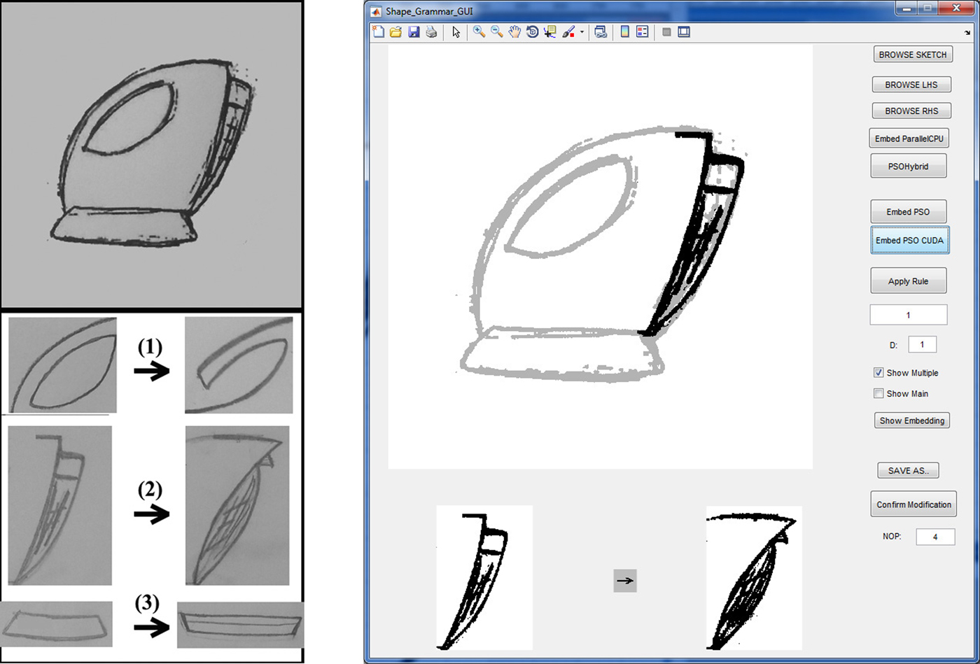
Fig. 3. Left: sample initial shape and rule shapes. Right: Application GUI that shows the embedding second rule in the kettle shape.
All the experiments presented here are performed on a machine that has Intel i7-4790K CPU and NVidia GeForce GTX 970 graphics card. The GPU implementation is run by setting the block number as the number of tiles and the number of threads in each block as the number of particles in each tile. In our initial tests, we used 1024 particles that are divided evenly for each block. Hence, if there are 16 tiles, that is, a 4 × 4 grid setting, each tile contains a swarm of 64 particles, that is, each block contains 64 threads. In our current CPU architecture, there are four CPU cores that can be run simultaneously as discussed in Keles, Reference Keles2015. Therefore, we performed the tests with 2 × 2 tiles setting to compare our single thread CPU, parallel CPU and GPU implementations (Table 1). When we set the number of particles fixed, the effect of tile configuration to the execution times is minimized.

Fig. 4. Sample derivations using the kettle shape.
Table 1. Execution times of the three PSO implementations using a total of 1024 particles during searches (2 × 2 tiles).
The performance of the GPU based PSO algorithm is depicted with bold lines.
In this table, we provide the performance values of the alternative implementations of the proposed method for the three considered examples. All three implementations, namely the serial CPU implementation, parallel CPU implementation and GPU implementation are based on the proposed PSO algorithm. The speedup of GPU-based implementation over CPU is between 133× and 190×; whereas over parallel CPU implementation is between 45× and 73×.
We also tested our GPU-based solution with a number of different tile configurations using a fixed number of particles in each tile, that is, 1024 (Table 2). All the tests are performed conservatively for 50 iterations, although accurate alignments are usually obtained around iteration 10. The execution times show that even if the LHS is large, as in the four kettles test, embedding is done in <1 s up to around 100 tiles. For relatively small LHS shapes, a GPU-based solution runs less than 1 s even for 256 tiles, for 50 iterations.
Table 2. Executions times of the CUDA-based PSO implementation for a number of different tile configurations using a total of 1024 particles during searches.
As we state in the previous sections, when we increase the number of particles in each swarm, design space exploration is more effective, yet computationally more expensive. Hence, there is a tradeoff between the alignment accuracy and execution time. We configured a number of additional experiments, in which we keep the number of particles in each tile fixed, hence increased the total number of particles in searches, to evaluate the performance of the GPU solution. In this case, the tiling configuration has a direct effect on the execution times. For example, if the search space is split into 16 tiles, there are 16 × 1024 particles in total. For this test, we used 2 × 2 tiles again so that we can compare the performances of the GPU implementation with our parallel CPU implementation. The results are depicted in Table 3. In the serial and parallel CPU implementations, the execution time increases around four times, compared with the fixed number of particles (Table 1). On the other hand, the increase in GPU implementation is on the average 1.8 times. These experiments show that our GPU-based implementation provides a significant amount of improvement in the execution times.
Table 3. Execution times of the three PSO implementations using 1024 particles in each block (2 × 2 tiles)
The performance of the GPU based PSO algorithm is depicted with bold lines.
In Figure 4, we present sample derivations using the kettle sketch depicted in Figure 3. The rules are applied in the given order. In order to keep the results compact, we present the resultant images, instead of repeating the GUI in each figure. On the first row, one kettle is used as the initial shape. The search space is represented as one tile and a swarm with 1024 particles searches the entire image region in cooperation to get the best candidate embedding. The embedded parts are depicted in bold lines, while the original image is shown slightly faded. The initial shape in the second row is composed of four identical kettle sketches. In this representation, the search space is represented with four tiles, each one contains 1024 particles, and best of each tile is selected as the embedded parts. The algorithm is run for 50 iterations for ten times in a row and the particles of each swarm were able to find the expected sub-shape alignments for each trial. The embedding computation takes around 0.36 s in our test machine, although there are 4096 number of particles that are computing the costly fitness function concurrently for 50 times. We believe that these results show the potential benefits of GPU–PSO-based parallel implementation both with respect to the quality of the computed transformation and execution time.
Alternatively, in order to maximize the utilization of the GPU resources, the image space in the first row is also divided into a number of tiles (i.e., 16 and 32), where multiple swarms search the space simultaneously. Each of them returns its best candidates; yet only some of them, which are located close to the solution region, can return a cost value close to zero. The other solutions are eliminated by checking the embedding cost for each particle. Proper alignments would result in lower costs. For example, the result depicted in Figure 5 is obtained by dividing the image into 16 × 16 tiles; each tile is searched by 1024 particles simultaneously (i.e., a total of 262,144 particles). There are 256 candidate solutions at the end of the run. In all these solutions, only two particles return an alignment with a cost <5% alignment error. Figure 5 depicts these two embeddings on the same image; that is, why the embedded sub-shape is thicker than the searched LHS shape. Embedding both candidates actually highlights the embedded part more, rather than corrupting it.

Fig. 5. Two candidate embeddings are shown together.
The performance of the algorithm is similar when nine kettles were used as the initial shape (Fig. 6). In this example, image space is divided into 3 × 3 tiles, and best candidate for each block is depicted simultaneously.
Fig. 6. The parallel embeddings of the nine kettle shapes.
Extensive searching of an image, which contains repeated patterns, results in different embedding options. Some of these results may inspire the user by depicting many simultaneous divisions and fusions and hence many context switches one after another. It enables many reinterpretations of the parts of a shape in a short time. This is found to be an important feature for creative design exploration (Goldschmidth, Reference Goldschmidt1991). In our application, we allow the user to select a subset of these candidate embeddings to be applied to the initial shape. A sample derivation that is generated this way is depicted in Figure 7. There are six pairs of images in this figure; each pair contains an embedding result and the result of the selected rule application. The pairs are ordered from left to right and top to bottom. The resultant visual computation is depicted on the bottom right of the figure.
Fig. 7. An initial shape and two shape rules are depicted on the top row. Embeddings and rule applications are shown in this order for the random application of two rules six times.
The reduced computation time enables running multiple swarms concurrently. Therefore, the user of this system, for example, a designer, may freely explore the design space very effectively. To support design space exploration in a more flexible way, the system may also be configured to accept partial part embeddings as candidate results, if it is returned as a solution by a swarm. Such a system has a potential for depicting part alignments with an implicit/hidden structure in the initial shape, which may help “seeing” in ambiguities. The reason is that when we decrease the accuracy of alignments, we increase the potential of ambiguous interpretations. A sample derivation that is generated this way is depicted in Figure 8.
Fig. 8. A sample derivation that is run with a more flexible embedding configuration.
The initial shape is composed of overlapping, hence interacting, circles in a structured fashion. Our system allows utilization of the ambiguity, caused by these interactions, by revealing hidden structures in every step of these rule applications. The depicted derivation is performed by representing the image space as 2 × 2 tiles; hence, we see at most four results in each run. Sometimes, the user selects only particular embeddings, that is, the bottom left image.
Conclusion
In this work, we proposed a novel working implementation of a GPU-based PSO algorithm to efficiently solve the emergent part embedding problem for shape grammars. The research presented here shows that the PSO method is effective for locating sub-shapes in an initial shape. In order to increase the possibility of locating all valid parts, we divide the search space into multiple tiles and initiated searches in each tile with separate swarms. The cost of alignment optimization by multiple swarms is high; to overcome this, we configured parallel searches using the programmable graphics hardware. As a result, the computation time is reduced significantly with the concurrency provided by the GPU architecture and CUDA programming environment. Moreover, the alignment accuracy is increased substantially by competing particles operating in smaller search regions.
Although the experimental results show desirable part embeddings, determination of the tile configuration and an optimum number of particles in each tile still requires further investigation. In this research, we set these parameters manually to observe and validate the effectiveness of the searches for time and alignment accuracy. Since the results are promising in both perspectives, we can focus on improving and automating the best configuration settings of parallel PSO approach, depending on the design space characteristics in the future.
Acknowledgments
We thank the anonymous reviewers for their constructive comments. This research is funded by Ankara University (Scientific Research Projects Grant 15H0443009).
Hacer Yalim Keles received her BS, MS, and PhD degrees in Computer Engineering Department from Middle East Technical University, Turkey, in 2002, 2005, and 2010, respectively. From 2000 to 2007 she worked as a researcher and senior researcher at the Scientific and Technological Research Council of Turkey. She is currently working as an Assistant Professor in the Computer Engineering Department of Ankara University. Her research interests primarily lie in shape grammars, computer vision, pattern recognition, and general purpose programming on GPUs.