


Impact Statement
The efficient design of wind or hydro-kinetic turbine arrays requires the analysis of multiple layouts for a range of flow conditions, with the goal of maximising the energy yield over the project lifespan. This process can be accomplished adopting analytical wake models as they provide a reasonable accuracy to predict the velocity field accounting for wake-to-wake interactions, as well as having a low computational overhead enabling layout optimisation. As power scales to the cube of velocities, i.e.  $P \propto U^3$, it is of utmost importance to develop wake models that represent accurately the wakes downstream of turbines. This paper introduces a new super-Gaussian and Gaussian wake models for vertical axis turbines (VATs) capable of capturing the three-dimensional shape and maximum velocity deficit of their wake, notably improving any existing VAT wake model. The adoption of these theoretical models for array design by industry and researchers will enable more reliable estimates of the optimal turbine spacing that maximise the energy yield, contributing to accelerate the development of this technology for renewable energy generation.
1. Introduction
In the global landscape of wind energy generation, all commercial-scale onshore and offshore wind farm projects comprise horizontal axis turbines (HATs) as a well established technology. Vertical axis turbines (VATs) are being developed at a slower pace with a remaining main challenge to prove their financial viability in large-scale projects, which is partly conditioned by the need to enhance their energy generation capabilities. The VATs offer a series of advantages over their HAT counterparts that can lead to innovative wind and hydro-kinetic energy projects, e.g. they can effectively harness energy from low-to-medium flow velocity ranges such as found in urban areas, rivers or tides, or be adopted in environmentally sensitive regions as their slower rotational speeds can reduce fish collision risk and noise (Reference Castro-Santos and HaroCastro-Santos & Haro, 2013).
The VAT rotor blades rotate with their rotational axis perpendicular to the incident flow direction, generating vortical structures during the upstroke rotation and interacting with these over the downstroke period. This complex flow dynamics depends on the operational regime accounted for by the tip-speed ratio (TSR), which relates the blades’ angular speed to the free-stream velocity; and the turbine's rotor geometric solidity, which indicates the proportion of swept perimeter occupied by the blades (Reference PosaPosa, 2020b). The VATs designed with low-solidity rotors operate at high TSR with the blades undergoing light dynamic stall, i.e. flow separation occurs for effective angles of attack larger than the static-stall angle. In contrast, rotors with higher solidity operate at low TSR and blades experience deep dynamic stall, meaning that leading-edge vortices enhance the blades’ lift-generation capability but eventually get fully detached originating a sudden drop in lift and torque, thus triggering large load fluctuations (Reference Ouro and StoesserOuro & Stoesser, 2017).
Despite the complex fluid--structure interaction, there is limited research looking into the governing flow mechanics of VAT wakes, especially in the far-wake region (Reference PosaPosa, 2020a). Most experimental tests of VATs look at how to improve their performance, leading to a limited number of studies analysing the near-wake flow field and fewer extensive tests investigating the far wake. Particularly for the latter, only a few small-scale laboratory studies exist, including: Reference Rolin and Porté-AgelRolin & Porté-Agel (Reference Rolin and Porté-Agel2018) measured with particle image velocimetry (PIV) up to 10 diameters ( $D_0$) downstream of a VAT analysing the mean and turbulent kinetic energy equations; Reference Araya, Colonius and DabiriAraya et al. (Reference Araya, Colonius and Dabiri2017) investigated the near- to far-wake transition for turbine rotors with different number of blades and TSRs using PIV to measure up to 11 $D_0$ downstream; and Reference Ouro, Runge, Luo and StoesserOuro et al. (Reference Ouro, Runge, Luo and Stoesser2019) measured the wake up to 14 $D_0$ downstream with an acoustic Doppler velocimeter, showing that remnants of the turbine-induced wake are still observed at such far distances downstream.
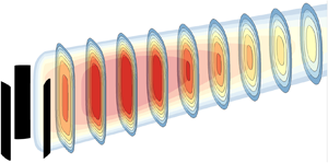
The uneven, three-dimensional distribution of VAT wakes is depicted in Figure 1, which considers a control volume (thick black lines) behind a turbine of diameter  $D_0$ and height $H_0$ in which mass and momentum need to be conserved (Reference Bastankhah and Porté-AgelBastankhah & Porté-Agel, 2014). Over the horizontal $xy$-plane, the main contribution to momentum entrainment over the lateral boundaries of the control volume results from blade-induced energetic vortices (Reference Kadum, Friedman, Camp and Bayoán CalKadum et al., 2018). This differs from the wake recovery dynamics over the $xz$-vertical plane (Figure 1b), as shear layers generated over this direction result from tip vortices (Reference Tescione, Ragni, He, Simão Ferreira and van BusselTescione et al., 2014). These blade-induced structures are not identical, contributing to a highly three-dimensional wake (Reference Ouro, Runge, Luo and StoesserOuro et al., 2019). Figure 1 shows that VAT rotors have two length scales that characterise the wake shape, namely $D_0$ is the characteristic length scale in the horizontal $xy$-plane while in the vertical $xz$-plane this is $H_0$.

Figure 1. Velocity deficit ( $\Delta U$) field behind a VAT of diameter $D_0$ and height $H_0$ over the (a) horizontal $xy$-plane at a mid-height elevation ( $z=z_h$) from the ground level, and (b) vertical $xz$-plane through the rotor's centre ( $y=\textit{0}$). Here, $k_y^*$ and $k_z^*$ are the wake expansion rates. Thick solid lines denote the control volume in which mass and momentum are conserved.
More insights into the complex turbulent structures generated by VAT rotor blades were gained from numerical simulations. Previous research has evidenced the need for eddy-resolving closures, e.g. large-eddy simulation (LES), to resolve this highly turbulent flow in order to capture dynamic stall (Reference Ouro, Stoesser and RamírezOuro et al., 2018) and estimate how turbulence drives the kinetic energy replenishment in the wake (Reference Bachant and WosnikBachant & Wosnik, 2016; Reference Ouro, Runge, Luo and StoesserOuro et al., 2019; Reference PosaPosa, 2020a). Geometry-resolved simulations provided of high grid resolutions at the rotor can capture the vortices induced by the blades (Reference Posa and BalarasPosa & Balaras, 2018; Reference Ouro and StoesserOuro & Stoesser, 2017). Actuator techniques capture the main wake dynamics while adopting coarser resolutions (Reference Porté-Agel, Bastankhah and ShamsoddinPorté-Agel et al., 2020), with the actuator line model (ALM) being the most adopted one (Reference Shamsoddin and Porté-AgelShamsoddin & Porté-Agel, 2016; Reference Abkar and DabiriAbkar & Dabiri, 2017; Reference Mendoza, Chaudhari and GoudeMendoza et al., 2019), although an improved resolution of the flow at rotor level can be obtained with actuator surface models (Reference Massie, Ouro, Stoesser and LuoMassie et al., 2019).
The drawback of high-fidelity LES–ALM is its large computational expense, becoming unfeasible to design array layouts (Reference Hezaveh, Bou-Zeid, Dabiri, Kinzel, Cortina and MartinelliHezaveh et al., 2018). Alternatively, analytical wake models represent the wake shape, normally adopting a top-hat, Gaussian or super-Gaussian distribution, enabling the optimisation of array layouts that provide the best performance throughout the project's lifespan (Reference Stansby and StallardStansby & Stallard, 2016; Reference Shapiro, Starke, Meneveau and GaymeShapiro et al., 2019). The adopted model needs to capture the velocity and length scales that define the wake in order to improve the results and diminish the uncertainty in the predictions (Reference Archer, Vasel-Be-Hagh, Yan, Wu, Pan, Brodie and MaguireArcher et al., 2018). For instance, for HAT wakes Gaussian shape functions provide good results for HATs with zero yaw angle as their wakes feature an axisymmetric distribution, allowing us to consider the velocity deficit field to be self-similar (Reference Stallard, Feng and StansbyStallard et al., 2015; Reference Bastankhah and Porté-AgelBastankhah & Porté-Agel, 2016). Recent wake models adopting super-Gaussian functions have been introduced for HATs, providing good results, especially in the near wake compared to standard Gaussian models. The former have an initial shape close to a top-hat distribution behind the turbine and evolve towards a nearly Gaussian shape further downstream (Reference Shapiro, Starke, Meneveau and GaymeShapiro et al., 2019; Reference Blondel and CathelainBlondel & Cathelain, 2020).
In the case of VATs, there is still a need for developing analytical wake models that can describe and predict the three-dimensional field (Reference MeneveauMeneveau, 2019), as the wake is three-dimensional and scales with the VAT rotor's diameter and height, unlike HAT wakes that scales with the diameter. Current theoretical VAT wake models do not account for the uneven wake expansion over the horizontal and vertical planes (Figure 1), and represent its shape with standard Gaussian functions (Reference Abkar and DabiriAbkar & Dabiri, 2017; Reference AbkarAbkar, 2019). To overcome these limitations, a super-Gaussian shape enables a more physically realistic description of the VAT wake velocity field compared to top-hat models that assume a uniform value across the wake or Gaussian models that fail to reproduce the elliptical shape (Reference Blondel and CathelainBlondel & Cathelain, 2020).
We present and validate two novel analytical models based on a new super-Gaussian function and an improved model that adopts a Gaussian function. The former is particularly suitable for VAT wakes as it enables us to represent the near wake with an almost top-hat distribution which evolves towards a nearly Gaussian shape in the far wake. It captures the elliptical wake shape with the superposition of two different super-Gaussian functions in the lateral and vertical directions. We also propose a Gaussian wake model that improves the initial wake width, overcoming the limitation found in previous VAT wake models to calculate the velocity deficit in the near-wake region. Our models are applicable to wind vertical axis turbines in zero-pressure flows and also to hydro-kinetic VATs if these operate in a boundless environment without considerable influence from free-surface proximity or channel lateral blockage (Reference Ross and PolagyeRoss & Polagye, 2020). For simplicity, we refer to either of these as VATs to generalise the models’ applicability.
2. Derivation of the Wake Models
2.1. Momentum Conservation
We build our momentum conserving wake models starting from the conservation form of the Reynolds-averaged Navier–Stokes (RANS) equations for high Reynolds numbers in the streamwise direction. After neglecting viscous terms and considering the wakes to be in zero-pressure gradient flow, e.g. not in a high blockage environment as a shallow tidal channel, the equation reads
 \begin{equation} \frac{\partial U_w (U_0 - U_w)}{\partial x} + \frac{\partial V_w (U_0 - U_w)}{\partial y} + \frac{\partial W_w (U_0 - U_w)}{\partial z} = \frac{\partial u'u'}{\partial x} + \frac{\partial u'v'}{\partial y} + \frac{\partial u'w'}{\partial z}, \end{equation}
with ( $U_w,V_w,W_w$) being the vector of mean wake velocities in the streamwise, transverse and vertical directions respectively, $U_0$ is the free-stream velocity and $u'u'$, $u'v'$ and $u'w'$ denote time-averaged turbulent fluctuation correlations. We integrate (1) at any streamwise location of a control volume that embeds the turbine and expands over the $y$ and $z$ directions from $-\infty$ to $\infty$, which together with the assumption that the shear stresses vanish when the distance from the wake centre increases, provides the resulting RANS equation:
 \begin{equation} \frac{\textrm{d}}{\textrm{d}\,x} \int_{-\infty}^{\infty} (U_{w}(U_{0} - U_{w}) -u'u')\,\mathrm{d} A \approx 0 . \end{equation}
 The streamwise variation of  $u'u'$ is much reduced when compared to the convective term (Reference Bastankhah and Porté-AgelBastankhah & Porté-Agel, 2014), hence (2) can be simplified to obtain the momentum integral (Reference Tennekes and LumleyTennekes & Lumley, 1972) as
 \begin{equation} \rho\int_{-\infty}^{\infty} (U_{w}(U_{0} - U_{w}))\,\mathrm{d} A = T. \end{equation}
 This equilibrium condition states that the momentum deficit flux in the wake is proportional to the thrust force  $T$ exerted by the turbine. The thrust force can be related to the thrust coefficient ( $C_T$) from the actuator disc theory as
 \begin{equation} T = \tfrac{1}{2}C_{T}\rho A_{0} U_{0}^2. \end{equation}
where  $\rho$ indicates the fluid density.
2.2. Top-hat Wake Distribution
Analogously to the Reference Frandsen, Barthelmie, Pryor, Rathmann, Larsen, Højstrup and ThøgersenFrandsen et al. (Reference Frandsen, Barthelmie, Pryor, Rathmann, Larsen, Højstrup and Thøgersen2006) top-hat HAT wake model, we assume the distance downstream of the rotor the flow in the wake required to reach the free-flow pressure is negligible. The cross-sectional area of the wake just after the initial wake expansion is considered rectangular as the turbine rotor's cross-sectional area at  $x=x_a$, i.e. $A_{w}(x_a)= A_{a}$. The value of the wake onset area $A_a$ can be determined using the actuator disc theory as $A_a = \beta A_0$, with $\beta$ representing the relative initial wake expansion at $x_a=0$ in terms of the turbine rotor's cross-section $A_0$, independently of whether such cross-section is circular (HATs) or rectangular (VATs). For a $C_T$ lower than the unity, the actuator disc theory states that the velocity over the plane at a downstream distance $x_a$ is $U_{0}(1-2a)$ whilst at the rotor centre plane the velocity is $U_{0}(1-a)$, with $a=(1-\sqrt {1-C_{T}})/2$ being the so-called induction factor. Hence, the value of $\beta$ is determined as
 \begin{equation} \beta = \frac{A_{a}}{A_{0}} = \frac{1-a}{1-2a} = \frac{1}{2}\frac{1 + \sqrt{1-C_{T}}}{\sqrt{1-C_{T}}}. \end{equation}
 The wake area at any streamwise location is determined similarly to the approach presented by Reference Frandsen, Barthelmie, Pryor, Rathmann, Larsen, Højstrup and ThøgersenFrandsen et al. (Reference Frandsen, Barthelmie, Pryor, Rathmann, Larsen, Højstrup and Thøgersen2006) for HATs with  $D_w \propto (x-x_a)^{1/2}$ and $H_w \propto (x-x_a)^{1/2}$, considering the wake width expands unevenly over the horizontal and vertical directions according to
 \begin{equation} D_{w} = D_0 \left(\beta + k_{w_{y}}\frac{x}{D_0}\right)^{1/2}, \quad H_{w} = H_0 \left(\beta + k_{w_{z}}\frac{x}{H_0}\right)^{1/2}. \end{equation}
 We now apply momentum balance to a control volume that embeds the operating turbine expanding some distance upstream and downstream to obtain the velocity deficit ( $\Delta U = U_0-U_w$) for the top-hat model with an uneven expansion over the horizontal and vertical directions
 \begin{equation} \frac{\Delta{U}}{U_{0}} = \frac{1}{2}\left(1-\sqrt{1-\frac{2 C_{T}}{ \left(\beta + k_{w_{y}}\dfrac{x}{D_0}\right)^{1/2} \left(\beta + k_{w_{z}}\dfrac{x}{H_0}\right)^{1/2} }}\right). \end{equation}
 Values of  $k_{w_y}$ and $k_{w_z}$ are the wake expansion rates in the $y$- and $z$-directions respectively, which can be calculated as 2.0 $I_u$ with $I_u= (u'u')^{0.5}/U_0$ being the streamwise turbulence intensity (Reference Frandsen, Barthelmie, Pryor, Rathmann, Larsen, Højstrup and ThøgersenFrandsen et al., 2006). In our study, we derived this top-hat wake model to estimate the initial wake width in the super-Gaussian and Gaussian models.
2.3. Super-Gaussian and Gaussian Wake Models
In the derivation of a super-Gaussian model, the wake is assumed to feature a velocity deficit ( $\Delta U$) distribution that evolves in the streamwise direction according to the local scale of velocity $C(x)$, determined as the maximum normalised velocity deficit ( $\Delta U_{max}/U_0$); and spatial length scales $f_y(y)$ and $f_z(z)$ that define an three-dimensional super-Gaussian distribution according to exponents $n_y$ and $n_z$, respectively. In the case of HATs (Reference Blondel and CathelainBlondel & Cathelain, 2020) or VATs, the wake starts with a rectangular (or nearly top-hat) shape immediately and evolves with an elliptical shape until attaining a Gaussian shape in the far wake ( $n_y = n_z = 2$) assuming it is self-similar (Reference Bastankhah and Porté-AgelBastankhah & Porté-Agel, 2014). Thus, $n_y$ and $n_z$ are deemed to vary in the streamwise direction following an exponential decay as
 \begin{equation} n_y = a_y \exp \left( - b_y \frac{x}{D_0} \right) + c_y, \quad n_z = a_z \exp \left( - b_z \frac{x}{H_0} \right) + c_z . \end{equation}
 Here, we denote the normalised local coordinates  $\tilde {y} = (y - y_c)/D_0$ and $\tilde {z} = (z-z_c)/H_0$, with $y_c=0$ and $z_c=z_h$ being the centre of the turbine's rotor (Figure 1). Our super-Gaussian model is derived considering an uneven evolution of the wake shape over the $y$- and $z$-directions, i.e. $a_y \neq a_z$ and $b_y \neq b_z$ as shown later in § 4. Note that, in (8), we propose that the evolution of the shape exponent over the $y$-direction scales with $D_0$ whilst in the vertical direction this is with $H_0$. The evolution of $\Delta U$ according to the superposition of super-Gaussian shapes $f_y$ and $f_z$ can be estimated as
 \begin{equation} \frac{\Delta U}{U_0} = \frac{U_0 - U_w}{U_{0}} = C(x) \exp \left( -\frac{\tilde{y}^{n_y}}{2\tilde{\sigma_y}^2} \right) \exp \left( -\frac{\tilde{z}^{n_z}}{2\tilde{\sigma_z}^2} \right). \end{equation}
 The characteristic wake widths  $\sigma _y$ and $\sigma _z$ again scale depending on $D_0$ and $H_0$, respectively, i.e. $\tilde {\sigma _y} = \sigma _y/D_0$ and $\tilde {\sigma _z} = \sigma _z/H_0$. These wakes grow linearly in the downstream direction according to the wake expansion rates $k_y^*$ and $k_z^*$ respectively, which read
 \begin{equation} \tilde{\sigma_y} = k_y^{ * } \frac{x}{D_0} + \varepsilon_{y} , \quad \tilde{\sigma_z} = k_z^{ * } \frac{x}{H_0} + \varepsilon_{z}, \end{equation}
with  $\varepsilon _y$ and $\varepsilon _z$ representing the initial wake expansion at $x_a$. In our model, the wake expansion rates are determined as a function of the streamwise turbulence intensity as $k_y^*=k_z^*=0.45I_u$, which are slightly greater than the values normally adopted for HAT. The wake velocity deficit (9) can be re-written as
 \begin{equation} U_{w} = U_{0}\left[ 1-C(x) \exp {\left(-\frac{\tilde{y}^{n_y}}{2 \tilde{\sigma_y}^2} \right)} \exp {\left(-\frac{\tilde{z}^{n_z}}{2 \tilde{\sigma_z}^2} \right)} \right] .\end{equation}
 We need to determine the velocity scale  $C(x)$ as the unknown variable from this algebraic equation. Considering the wake area to be $A_w=D_w H_w$ ( $\textrm {d}A=\textrm {d}y\,\textrm {d}z$) depicted in Figure 1, we equate the momentum integral (3) to the turbine thrust force (4) to obtain the definition of the wake velocity (11) as
 \begin{equation} \int_{-\infty}^{\infty} \int_{-\infty}^{\infty} C(x) \exp {\left(-\frac{\tilde{y}^{n_y}}{2 \tilde{\sigma_y}^2}-\frac{\tilde{z}^{n_z}}{2 \tilde{\sigma_z}^2}\right)}\left[1-C(x) \exp {\left(-\frac{\tilde{y}^{n_y}}{2 \tilde{\sigma_y}^2}-\frac{\tilde{z}^{n_z}}{2 \tilde{\sigma_z}^2}\right)}\right] \mathrm{d} y\,\mathrm{d} z = \frac{1}{2}C_{T} A_{0}. \end{equation}
 In the integration of (12) we consider that  $\int _{-\infty }^{\infty } \exp (-\tilde {y}^{n_y}/(2 \tilde {\sigma _y}^2) \,\textrm {d}y$ = $2/n_yD_0 \varGamma (1/n_y)(2\tilde {\sigma _y}^2)^{1/n_y}$, $\int _{-\infty }^{\infty } \exp (-\tilde {y}^{n_y}/\tilde {\sigma _y}^2) \,\textrm {d}y = 2/n_yD_0 \varGamma (1/n_y) \tilde {\sigma _y}^{2/n_y}$, and analogously for the integrals in $z$-direction, with $\varGamma (1/2) = \sqrt {{\rm \pi} }$ and $\varGamma (1) = 1$. For convenience, from hereafter we denote $\eta$ = 1/ $n_y$+1/ $n_z$. Equation (12) can be integrated to determine the normalised maximum velocity deficit, $C(x)$, as
 \begin{equation} C(x)^2 - C(x) 2^\eta + \frac{C_T n_y n_z}{8 \tilde{\sigma_y}^{2/n_y}\tilde{\sigma_z}^{2/n_z} \varGamma(1/n_y) \varGamma(1/n_z)} = 0. \end{equation}
From the two possible roots of this quadratic equation, the solution that provides a physically acceptable value for the characteristic velocity scale is
 \begin{equation} C(x) = 2^{\eta-1} - \sqrt{2^{2\eta-2} - \frac{C_T n_y n_z}{8 \tilde{\sigma_y}^{2/n_y}\tilde{\sigma_z}^{2/n_z} \varGamma(1/n_y) \varGamma(1/n_z)} }. \end{equation}
Hence, our super-Gaussian model for VAT wakes is determined from (11) and (14) as
 \begin{equation} \frac{\Delta{U}}{U_{0}} = \left( 2^{\eta-1} - \sqrt{2^{2\eta-2} - \frac{C_T n_y n_z}{8 \tilde{\sigma_y}^{2/n_y}\tilde{\sigma_z}^{2/n_z} \varGamma(1/n_y) \varGamma(1/n_z)}} \right) \left[ \exp {\left(-\frac{\tilde{y}^{n_y}}{2 \tilde{\sigma_y}^2} \right)} \exp {\left(-\frac{\tilde{z}^{n_z}}{2 \tilde{\sigma_z}^2} \right)} \right]. \end{equation}
 Note that if a Gaussian velocity profile is considered for both  $f_y$ and $f_z$, i.e. $n_y=n_z=2$, then $\tilde {y}^2/ \tilde {\sigma _y}^2 = y^2/\sigma _y^2$ and $\tilde {z}^2/ \tilde {\sigma _z}^2 = z^2/\sigma _z^2$, yielding a velocity deficit expression
 \begin{equation} \frac{\Delta{U}}{U_{0}} = \left( 1- \sqrt{1-\frac{C_{T}A_{0}}{2{\rm \pi}\sigma_{y}\sigma_{z}}} \right) \left[ \exp {\left(-\frac{{y}^2}{2 {\sigma_y}^2} \right)} \exp {\left(-\frac{z^2}{2 {\sigma_z}^2} \right)} \right]. \end{equation}
2.3.1. Initial Wake Width
We need to determine the initial wake width to estimate the values of  $\varepsilon _y$ and $\varepsilon _z$ adopted in the calculation of the wake widths $\tilde {\sigma }_y$ and $\tilde {\sigma }_z$. These are determined from the mass flow deficit rate ( $m = \rho \iint \Delta U \,\textrm {d}A$, with $\rho$ being the density of the fluid) immediately behind the turbine's rotor $x=0$, equating the prediction from the momentum-conserving top-hat model (7) to the value from the super-Gaussian model (15), which ensures mass and momentum are conserved over the wake width. The expression of mass flow deficit rate for the super-Gaussian wake model reads
 \begin{equation} m_{{SG}} = \left( 2^{\eta-1} - \sqrt{2^{2\eta-2} - \frac{C_T n_y n_z}{8 \varepsilon_y^{{2}/{n_y}} \varepsilon_z^{{2}/{n_z}} \varGamma({1}/{n_y}) \varGamma({1}/{n_z}) }} \right) \frac{D_0H_0 2^{\eta + 2} \varepsilon_y^{{2}/{n_y}} \varepsilon_z^{{2}/{n_z}} \varGamma({1}/{n_y}) \varGamma({1}/{n_z}) }{n_yn_z}. \end{equation}
Alternatively, the mass flow deficit rate from the top-hat model (7) is
 \begin{equation} m_{{TH}_{x = 0}} = \left(1-\sqrt{1-\frac{2C_{T}}\beta} \right) \frac{D_a H_a}{2}. \end{equation}
 Considering the wake onset widths  $\varepsilon _y$ and $\varepsilon _z$ are equal to $\varepsilon$, we obtain
 \begin{equation} \varepsilon (n_{y,z}\geq 2) = \left( \frac{\beta n_yn_z}{2^{2\eta + 2} \varGamma\left({1}/{n_y}\right) \varGamma\left({1}/{n_z}\right)} \right)^{1/(2\eta)}. \end{equation}
 It should be noted that these values of  $n_y$ and $n_z$ are those at $x=0$, as $\varepsilon _y$ and $\varepsilon _z$ are solely evaluated as the initial wake width. The initial wake width adopting a Gaussian distribution is
 \begin{equation} \varepsilon (n_{y,z} = 2) = \sqrt{\frac{\beta}{4{\rm \pi}}}. \end{equation}
 The initial wake expansion rates are just a function of  $\beta$, i.e. only depend on the thrust coefficient $C_T$. It is noteworthy that our estimation of the initial wake width using a super-Gaussian model (19) differs from the definition $\varepsilon = \sqrt {\beta }/4$ proposed by Reference Abkar and DabiriAbkar & Dabiri (Reference Abkar and Dabiri2017) which is approximately 12% smaller and corresponds to the value used in HAT wake models. Our formulation overcomes limitations derived from an inaccurate definition of $\varepsilon$ which can yield non-physical estimations of the velocity deficit at short distances behind the turbines. Furthermore, the velocity scale obtained in our Gaussian model (16) differs from that proposed in Reference Abkar and DabiriAbkar & Dabiri (Reference Abkar and Dabiri2017), as the latter assumed the velocity deficit at the wake onset to be that of HATs (Reference Bastankhah and Porté-AgelBastankhah & Porté-Agel, 2014), while our theoretical framework is derived considering the rectangular section of VAT rotors. This consideration, together with the initial wake width (20), allows us to compute the velocity deficit field at any downstream location for any $C_T$ and rotor aspect ratio. In Table 1 we present the values of the super-Gaussian wake model (19) parameters, which provided the lowest error in the velocity predictions, and wake recovery rates used in the Gaussian model. The computed root-mean-square error in the velocity predictions shown later in Section 4 varied less than 2% when decreasing or increasing the super-Gaussian model input parameters $a_y$, $a_z$, $b_y$ and $b_z$ by $\pm$20%, similarly to the sensitivity analysis presented in Reference AbkarAbkar (Reference Abkar2019) for a Gaussian model.
Table 1. Details of the parameters adopted in the super-Gaussian and Gaussian wake models.

3. Evolution of the Wake Shape with Varying Aspect Ratio
A key aspect that can be elucidated with our three-dimensional super-Gaussian model is whether VAT wakes ever become circular (i.e. axisymmetric) and, if so, at what distance downstream the turbine is this accomplished? The evolution from an elliptical shape converging into a circular one was observed by Reference Shamsoddin and Porté-AgelShamsoddin & Porté-Agel (Reference Shamsoddin and Porté-Agel2020) using LES for three rotor aspect ratios. According to (8), the evolution of the shape function exponents  $n_y$ and $n_z$ scale with $D_0$ and $H_0$ respectively, thus the downstream distance at which symmetry in the wake shape is accomplished depends on the aspect ratio $\xi = H_0/D_0$. This is irrespective of the wake recovery rate that is a linear function of $k_y^*$ and $k_z^*$, which are both equal and only a function of turbulence intensity (Table 1).
We present the downstream evolution of the ratio  $n_z/n_y$ for different aspect ratios in Figure 2 to identify whether the wake shape is elliptical (asymmetric) or circular (i.e. $n_z$= $n_y$). As presented in Figure 11 in the Appendix, at the wake onset, the exponents $n_y (x=0)$ and $n_z (x=0)$ approach 3.35 and 6.9 respectively, representing top-hat-like shape functions, yielding an initial value $n_z/n_y (x=0)$ equal to 2.060. Further downstream these eventually converge towards a value of 2.4, i.e. $n_z/n_y$ = 1.0, similarly to other HAT super-Gaussian models (Reference Shapiro, Starke, Meneveau and GaymeShapiro et al., 2019; Reference Blondel and CathelainBlondel & Cathelain, 2020). For a square-shaped rotor, i.e. $\xi = 1$, the near wake is characterised by $n_z$ being larger than $n_y$ until $x/D_0 \approx 4.0$, when a reversed shape is developed, and not until approximately 10 $D_0$ is a symmetric (circular) wake recovered. For $\xi \geq 1.5$, the ratio $n_z/n_y$ remains larger than 1.0 at all streamwise distances, indicating that the wake requires a longer streamwise distance to recover the Gaussian shape over the vertical direction that in the lateral one. Thus, increasing the aspect ratio progressively increases the downstream distance required to recover wake symmetry, and for $\xi \geq 5.0$ the maxima of the $n_z/n_y$ ratio are not attained at the wake onset but instead at some distance downstream $x$ up to which $n_z$ evolves notably slower than $n_y$ (Figure 11). Conversely, for $\xi \leq 1.5$ the asymmetry in the near wake comes from $f_z$ evolving faster towards a nearly Gaussian distribution than $f_y$, with the circular shape attained after approximately 10–12 $D_0$, equivalent to 64 $H_0$ for $\xi = 0.25$. Our super-Gaussian theoretical model indicates that a symmetric circular shape is recovered fastest with $\xi = 1.5$ (specifically at $x/D_0 = 10$), as this is the threshold value at which the wake in the vertical direction never approaches the Gaussian shape at a faster rate than over the horizontal plane.

Figure 2. Evolution of wake shape accounted for by the ratio  $n_z/n_y$, with schematics of the wake shape on the left-hand side.
4. Validation of the Wake Models
We validate our theoretical wake models in six cases comprising a single VAT operating in the turbulent atmospheric boundary layer flow with comparisons to high-fidelity LES. Cases 1a, 1b and 1c reproduce the LES from Reference Shamsoddin and Porté-AgelShamsoddin & Porté-Agel (Reference Shamsoddin and Porté-Agel2020) which change the turbine rotor's aspect ratio ( $\xi$) from 2.0 to 0.25, whilst keeping the incident flow characteristics and turbine operation constant. Cases 2a and 2b consider the set-up and LES results presented in Reference Abkar and DabiriAbkar & Dabiri (Reference Abkar and Dabiri2017) in which the VAT rotor's diameter and height are kept constant ( $\xi =0.92$) but thrust coefficients are lower than in cases 1a to 1c. For completeness, case 2c is also included despite its aspect ratio is close to case 1b but the thrust coefficient is smaller. These benchmarks are selected as they provide the necessary information to input in the analytical models, i.e. approach velocity characteristics (e.g. free-stream velocity, $U_0$, and turbulence intensity, $I_u$), rotor dimensions and, more importantly, thrust coefficient (see Table 2 for details). Hereafter, the origin of coordinates is at the turbine rotor's centre of rotation and mid-height, and for simplicity the turbine rotor's diameter and height are represented by $D$ and $H$ instead of $D_0$ and $H_0$.
Table 2. Details of the cases tested, including VAT rotor's diameter  $D$, height $H$ and aspect ratio $\xi$, height above ground of the turbine's centre $z_h$, thrust coefficient $C_T$, free-stream velocity $U_0$, streamwise turbulence intensity $I_u$ and TSR $\lambda$.

4.1. Case 1: VAT of Varying Aspect Ratio from Shamsoddin & Porté-Agel (Reference Shamsoddin and Porté-Agel2020)
Our super-Gaussian and Gaussian theoretical wake models are firstly validated for the three full-scale VATs of different aspect ratio originally presented in Reference Shamsoddin and Porté-AgelShamsoddin & Porté-Agel (Reference Shamsoddin and Porté-Agel2020) which used LES–ALM. The approach flow follows a logarithmic distribution with a roughness height of 0.1 m and friction velocity equal to 0.52 m s $^{-1}$ (Reference Shamsoddin and Porté-AgelShamsoddin & Porté-Agel, 2016). In Figure 3 we present the horizontal ( $y$) and vertical ( $z$) profiles of the normalised velocity deficit, $\Delta U$, at streamwise locations $x/D = 1$, 3, 5, 7 and 9 for case 1a ( $\xi =1.0$). There is a notable three-dimensionality in the near wake at $x/D = 1$, with the vertical profile featuring a top-hat-like shape whilst the wake shape in the $y$-direction is closer to a Gaussian distribution. Here, the super-Gaussian wake model captures well both the wake shape and maximum velocity deficit. In contrast, the Gaussian model estimates well the velocity deficit in the centre of the wake but is unable to reproduce the wake shape. The profiles at $x/D=3$ show that both models underestimate the velocity deficit at this location. At $x/D \geq 5$, the super-Gaussian model agrees well with the LES results, while the Gaussian model underestimates the velocity deficit magnitude, except for $x/D=9$ in which there is a good agreement.

Figure 3. Normalised velocity deficit profiles for case 1a with  $C_T = \textit{0.80}$ and $\xi = \textit{1.0}$. Comparison of our proposed super-Gaussian (red line) and Gaussian (black line) analytical wake models, with LES results from Reference Shamsoddin and Porté-AgelShamsoddin & Porté-Agel (Reference Shamsoddin and Porté-Agel2020) (circles).
The results for case 1b with  $\xi = 2.0$ are presented in Figure 4 at the same downstream sections as in Figure 3, with the profiles nearer to the VAT exhibiting a more pronounced top-hat distribution. Compared to LES, a larger wake width is predicted by the super-Gaussian model at $x/D$ = 1, likely due to an over-estimation of the initial wake width value $\varepsilon$ (similarly to the results obtained in the Gaussian model derivation for HATs by Reference Bastankhah and Porté-AgelBastankhah & Porté-Agel (Reference Bastankhah and Porté-Agel2014) in which a one-fifth reduction of $\varepsilon$ yielded better results), or from the influence of the proximity of the turbine bottom tip to the ground surface that generates flow acceleration ( $\Delta U \leq 0$) which is not captured in the wake models. Nevertheless, the super-Gaussian model yields a good prediction of the wake width in the vertical profiles further downstream as well as in the rest of the cases analysed, i.e. captures well the wake evolution over the horizontal and vertical directions. In cases 1a and 1b, an uneven wake shape is observed in the far wake at $x/D$ = 9, agreeing with the evolution of the ratio $n_z/n_y$ presented in Figure 2, with a symmetric (or circular) wake shape attained at $x/D \approx 16$ and 32 for $\xi = 1.0$ and 2.0, respectively.

Figure 4. Normalised velocity deficit profiles for case 1b with  $C_T = \textit{0.80}$ and $\xi = \textit{2.0}$. Same legend as Figure 3.
Case 1c considers a turbine with a small aspect ratio of 0.25, i.e. the VAT rotor's height is four times smaller than its diameter. Wake predictions from our theoretical models presented in Figure 5 evidence that the super-Gaussian model is able to accurately predict the near and far wakes. However, the Gaussian model underestimates the maximum velocity deficit in the near wake for  $x/D \leq 3$ but attains a good accuracy further downstream as the wake becomes nearly symmetric after $x/D = 7$, in agreement with Figure 2. The presented results show that VAT wakes evolve from an elliptical distribution to a circular one. This is observed in Figure 6, with contours of velocity deficit over $yz$-planes at several streamwise locations for cases 1a ( $\xi =1.0$) and 1b ( $\xi =2.0$), only showing values of $\Delta U/U_0 \geq 0.05$. With $\xi = 1.0$, the wake immediately downstream of the turbine remains wider in the vertical direction. At $x/D = 2$, its shape is almost symmetric whilst at $x/D = 5$ the wake has a larger extent in the transverse direction, reaching an almost circular shape at 10 $D$. As per the case with $\xi = 2.0$, the wake is highly three-dimensional at all locations, progressively evolving towards a circular shape.

Figure 5. Normalised velocity deficit profiles for case 1c with  $C_T = \textit{0.80}$ and $\xi = \textit{0.25}$. Same legend as Figure 3.

Figure 6. Velocity deficit contours over  $yz$-planes at various streamwise locations for cases 1a (top) and 1b (bottom) which depict the evolution of the wake from an elliptical to a circular shape, as indicated in Figure 2. Shaded area represents the VAT rotor's cross-section.
4.2. Case 2: VATs with Varying  $C_T$ from Abkar & Dabiri (Reference Abkar and Dabiri2017)

We now consider another LES set-up comprising a single VAT with  $D = 26$ m and $H = 24$ m, i.e. $\xi = 0.92$, operating at TSRs, $\lambda$, of 3.8 (case 2a) and 2.5 (case 2b). In these operating conditions, the VAT yields $C_T$ equal to 0.64 and 0.34, and we are interested in comparing these as VAT wakes develop a different dynamics depending on $\lambda$. Furthermore, in case 2c the turbine has a $C_T$ equal to 0.64 and operates at $\lambda = 3.8$, as in case 1a, but with $\xi = 1.85$. Turbines are equipped with three NACA 0018 blades with a chord length $c = 0.75$ m.
The validation of normalised velocity deficit predictions obtained with our analytical wake models compared with LES results from Reference Abkar and DabiriAbkar & Dabiri (Reference Abkar and Dabiri2017) are presented in Figure 7 with horizontal and vertical profiles across the turbine wake centre at  $x/D = 1$, 3, 6, 9 and 12. Immediately downstream the VAT, at $x/D =1.0$, the super-Gaussian model is able to capture the three-dimensional wake with the Gaussian model predicting a narrower wake core. At $x/D = 3$, the super-Gaussian model achieves excellent agreement with the LES data whilst the Gaussian model slightly under-predicts $\Delta U/U_0$ in both vertical and horizontal profiles. At locations further downstream, both models predict well the velocity deficit.

Figure 7. Normalised velocity deficit profiles for case 2a with  $C_T = \textit{0.64}$, $\lambda = \textit{3.8}$ and $\xi = \textit{0.92}$. Comparison of our proposed super-Gaussian (red line) and Gaussian (black line) analytical wake models, with the LES results from Reference Abkar and DabiriAbkar & Dabiri (Reference Abkar and Dabiri2017) (circles).
Figure 8 presents the results obtained for case 2b in which the VAT has a lower  $C_T$ than cases 2a and 2c. The super-Gaussian model again attains a good velocity field prediction at all locations, notably improving the velocity estimates from the Gaussian model, especially at $x/D = 3$ and 6, but both provide a reasonable agreement of the wake width. Due to the low $C_T$ in case 2b, the wake shape features an almost Gaussian distribution over the horizontal and vertical directions already at $x/D \geq 6$, which supports the self-similarity assumption in the Gaussian shape distribution and thus both theoretical models achieve a great accuracy.

Figure 8. Normalised velocity deficit profiles for case 2b with  $C_T = \textit{0.34}$, $\lambda = \textit{2.5}$ and $\xi = \textit{0.92}$. Same legend as Figure 7.
The turbine in case 2c has almost the same aspect ratio as in case 1b but with a lower thrust coefficient, which would lead to a faster wake recovery. Profiles of velocity deficit are shown in Figure 9 evidencing the accuracy of the super-Gaussian model in capturing the velocity deficit magnitude and its shape throughout the wake, notably improving the Gaussian model's prediction in the near wake at  $x/D = 3$. The wake is observed to expand unevenly over the vertical and horizontal directions as in Figure 4, but the wake recovery is faster for $C_T = 0.64$ than with $C_T = 0.80$, as would be expected.

Figure 9. Normalised velocity deficit profiles for case 2c with  $C_T = \textit{0.64}$, $\lambda = \textit{3.8}$ and $\xi = \textit{1.85}$. Same legend as in Figure 7.
4.3. Prediction of the Velocity Scale
To summarise the accuracy of our theoretical models in terms of the predictions of VAT wakes for the six cases analysed in comparison to LES results, the values of maximum velocity deficits in the streamwise direction are presented in Figure 10, which represents the velocity scale in the theoretical models (15). Overall, the super-Gaussian model attains an excellent agreement with LES in cases 1c, 2a, 2b and 2c over the whole wake length, whilst for cases 1a and 1b there is an underestimation of the velocity deficit until  $x/D \approx 5$, as a consequence of the models over-predicting the wake width (see Figure 7). The Gaussian model consistently provides good estimates of $\Delta U$ in the far wake but fails to achieve a good agreement in the near wake. Whilst further improvement in cases 1a and 1b would be obtained tuning the super-Gaussian parameters, we aimed at building a consistent model with a given set of parameters that yields the best predictions for the six benchmarks together. A further advantage of our Gaussian model is that the proposed initial wake width (20) enables the calculation of the velocity field in all the wake region, overcoming the limitations from previous models (Reference AbkarAbkar, 2019) that could not provide physical estimates in the near wake for ranges of $C_T$ values.

Figure 10. Evolution of the maximum normalised maximum velocity deficit in the streamwise direction for all cases analysed. Comparison of our proposed super-Gaussian (red line) and Gaussian (black line) wake models, with the LES results (circles) from Reference Shamsoddin and Porté-AgelShamsoddin & Porté-Agel (Reference Shamsoddin and Porté-Agel2020) in cases 1a to 1c and Reference Abkar and DabiriAbkar & Dabiri (Reference Abkar and Dabiri2017) in cases 2a to 2c.

Figure 11. Evolution of the super-Gaussian coefficients  $n_z$ and $n_y$ in the downstream direction for various aspect ratios $\xi = H/D$.
5. Conclusions
We present a new set of theoretical super-Gaussian and Gaussian models for vertical axis wind and hydro-kinetic turbine (VAT) wakes that capture their intrinsic three-dimensional shape. Our super-Gaussian model is based on the superposition of two super-Gaussian shape functions that evolve in the downstream direction according to the exponents  $n_y$ and $n_z$ which scale with the rotor's diameter ( $D$) and height ( $H$), respectively. This model represents well the nearly top-hat near-wake shape and elliptical distribution found along most of the wake length until it eventually collapses into an axisymmetric circular shape. The ratio between the shape function exponents indicates the degree of horizontal-to-vertical wake shape asymmetry (which varies with the rotor's height-to-diameter aspect ratio ( $\xi = H/D$) but is invariant to the flow conditions) showed that the fastest recovery to an axisymmetric wake was obtained for $\xi = 1.5$ at a distance of 8 $D$ downstream. Our Gaussian model considers the wake to be self-similar and yielded reliable estimates of the initial wake width but was less accurate in the near-wake representation than its super-Gaussian counterpart. In both models the wake width increases linearly as a function of turbulence intensity at the same rate in the vertical and transverse directions.
We validated the accuracy of our models with high-fidelity LES data in six cases involving a standalone VAT with varying thrust coefficients and aspect ratios. Our models captured the three-dimensional wake distribution, yielding good estimates of the maximum velocity deficit, with the super-Gaussian model providing the best predictions. The transition from an elliptical to a circular Gaussian shape is well captured by the super-Gaussian model, which indicated this is attained at a downstream location depending on the VAT's rotor aspect ratio, in line with the results previously observed in the LES. The presented results confirm the accuracy and reliability of our super-Gaussian model in the prediction of VAT wakes both in the near and far regions, while our Gaussian model represents well the far wake.
Acknowledgements
Authors are grateful to V. Muhawenimana and S. Mueller for fruitful discussions about this work, and the reviewers for their valuable comments that helped us to improve our work.
Funding Statement
This research was partially supported by the UK's Engineering and Physical Sciences Research Council (EPSRC) (EP/R51150X/1).
Declaration of Interests
The authors report no conflict of interest.
Appendix
As VAT wakes have two length scales, namely  $H$ and $D$, that determine their shape, in Figure 11 we show the change in the super-Gaussian coefficients $n_z$ and $n_y$ (8) with downstream distance. At $x/D$, both coefficients reach their maxima ( $n_z = 6.9$ and $n_y = 3.35$) corresponding to the most top-hat-like shape, then decaying exponentially until the Gaussian shape of exponent 2.4. We observe that for $\xi \leq 1.5$ the vertical wake shape eventually evolves quicker to the limit value of 2.4, whilst above that value the wake always recovers the Gaussian distribution faster over the horizontal $y$-direction. In Figure 2 we characterised the wake asymmetry as the ratio $n_z/n_y$, which attained a maximum value at the wake onset ( $x/D=0$) except when $\xi \geq 4.0$ when this is achieved shortly downstream from the turbine. Figure 11 indicates that the latter happens because the wake in the lateral direction ( $n_y$) changes more rapidly from the initial top-hat to the Gaussian shape than over the vertical direction.


 Open access