


Impact Statement
One method that climate scientists use to find structures in environmental data is unsupervised classification, where a machine learning model sorts data, such as temperatures from different parts of the ocean, into groups or classes. This paper proposes a new way of determining if an unsupervised classification model has “over-fit” the data available, which means it is using too many classes. This method will be useful for climate scientists using unsupervised classification for studying climate model data, as current criteria commonly used often don’t provide an upper limit on the number of classes.
1. Introduction
Studies using observational data of the climate system often seek to find structures within that data. Specifically, classifying complex data into coherent groups with similar properties is often the first step in a study that may seek to, for example, find borders between groups, describe the behavior of each group, explain the differences between the groups, or track changes in groups over time.
Unsupervised classification methods, that is, methods that do not know a priori what the properties of these groups might be, have proven adept at identifying coherent spatial structures within climate data, even when no spatial information is supplied to the algorithm. In studies of ocean and atmospheric data, two commonly used unsupervised classification methods are k-means (Solidoro et al., Reference Solidoro, Bandelj, Barbieri, Cossarini and Fonda Umani2007; Hjelmervik and Hjelmervik, Reference Hjelmervik and Hjelmervik2013; Reference Hjelmervik and Hjelmervik2014; Hjelmervik et al., Reference Hjelmervik, Hjelmervik and Østenstad2015; Sonnewald et al., Reference Sonnewald, Wunsch and Heimbach2019; Houghton and Wilson, Reference Houghton and Wilson2020; Yuchechen et al., Reference Yuchechen, Lakkis, Caferri, Canziani and Muszkats2020; Liu et al., Reference Liu, Chen, Chen, Chen, Ma and Meng2021) and Gaussian mixture modeling (GMM) (Hannachi and O’Neill, Reference Hannachi and O’Neill2001; Hannachi, Reference Hannachi2007; Tandeo et al., Reference Tandeo, Chapron, Ba, Autret and Fablet2014; Maze et al., Reference Maze, Mercier and Cabanes2017a; Jones et al., Reference Jones, Holt, Meijers and Shuckburgh2019; Crawford, Reference Crawford2020; Sugiura, Reference Sugiura2021; Zhao et al., Reference Zhao, Guo, Guo, Lin and Zhu2021; Fahrin et al., Reference Fahrin, Jones, Wu, Keeble and Archibald2022). K-means attempts to find coherent groups by “cutting” the abstract feature space using hyperplanes, whereas GMM attempts to represent the underlying covariance structure in abstract feature space using a linear combination of multi-dimensional Gaussian functions.
However, when dealing with highly-correlated data such as climate model output, the number of classes into which the data should be divided is not necessarily obvious; it remains a relatively unconstrained free parameter, and the classification methods themselves do not typically provide a way of choosing the “best” or most appropriate number of classes to describe a given dataset. In practice, most studies repeat the training of the model multiple times for different numbers of classes before applying a statistical criterion to compare the models. Statistical criteria alone do not always show a clear single “best” model, and so domain expertise is often additionally used to determine the appropriate number of classes for a given study.
The most commonly used statistical criterion is the minimum in the Bayesian information criterion (BIC; Schwarz, Reference Schwarz1978), used in Fahrin et al. (Reference Fahrin, Jones, Wu, Keeble and Archibald2022), Sugiura (Reference Sugiura2021), Zhao et al. (Reference Zhao, Guo, Guo, Lin and Zhu2021), Jones et al. (Reference Jones, Holt, Meijers and Shuckburgh2019), Maze et al. (Reference Maze, Mercier, Fablet, Tandeo, Lopez Radcenco, Lenca, Feucher and Le Goff2017b), Hjelmervik and Hjelmervik (Reference Hjelmervik and Hjelmervik2013, Reference Hjelmervik and Hjelmervik2014), Hjelmervik et al. (Reference Hjelmervik, Hjelmervik and Østenstad2015), and Sonnewald et al. (Reference Sonnewald, Wunsch and Heimbach2019). The BIC is comprised of two terms: a term that rewards the statistical likelihood of the model and a term that penalizes overfitting. One looks for a minimum or plateau in BIC in order to find the number of classes that maximizes statistical likelihood without overfitting.
Other common statistical methods used to compare clustering results by class number include the following (a nonexhaustive list):
-
• Akaike information criterion (AIC; Akaike, Reference Akaike, Petrov and Caski1973), used in Tandeo et al. (Reference Tandeo, Chapron, Ba, Autret and Fablet2014) and Sonnewald et al. (Reference Sonnewald, Wunsch and Heimbach2019).
-
• Caliński and Harabasz (Reference Caliński and Harabasz1974), used in Yuchechen et al. (Reference Yuchechen, Lakkis, Caferri, Canziani and Muszkats2020).
-
• Davies–Bouldin index (DBI; Davies and Bouldin, Reference Davies and Bouldin1979), used in Solidoro et al. (Reference Solidoro, Bandelj, Barbieri, Cossarini and Fonda Umani2007),
-
• Silhouette coefficient (Rousseeuw, Reference Rousseeuw1987), used in Houghton and Wilson (Reference Houghton and Wilson2020),
-
• criteria based on confidence intervals, used in Hannachi (Reference Hannachi2007).
-
• other scores based on log-likelihoods, used in Hannachi and O’Neill (Reference Hannachi and O’Neill2001) and Crawford (Reference Crawford2020),
Studies such as Liu et al. (Reference Liu, Chen, Chen, Chen, Ma and Meng2021) use physical justifications only.
Most of the studies cited above use unsupervised classification on observational data. One natural extension of a study based on observational data is to carry out a similar study based on data from numerical simulations. Possibilities include assessing the simulation’s fidelity, as well as greatly expanding the scope of the questions that can be asked, such as how robust clustering results are between different ensemble members, and how cluster properties vary in different simulated scenarios.
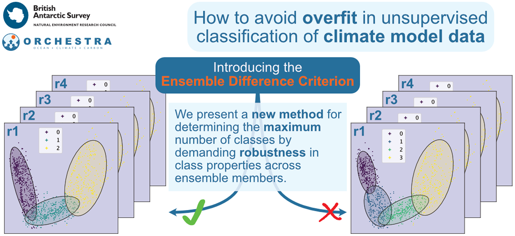
Given the rapid growth of clustering studies in recent years, and the many possibilities outlined above for motivating the use of simulated data, we believe that there will be a growing number of studies applying clustering techniques to simulated climate data. The use of multiple ensemble members is often required to reduce uncertainty due to internal variability (Deser et al., Reference Deser, Lehner, Rodgers, Ault, Delworth, DiNezio, Fiore, Frankignoul, Fyfe, Horton, Kay, Knutti, Lovenduski, Marotzke, McKinnon, Minobe, Randerson, Screen, Simpson and Ting2020), especially at regional or decadal scales where there is generally a lower signal to noise ratio (see, for example, Dosio et al., Reference Dosio, Jones, Jack, Lennard, Nikulin and Hewitson2019; Yeager et al., Reference Yeager, Danabasoglu, Rosenbloom, Strand, Bates, Meehl, Karspeck, Lindsay, Long, Teng and Lovenduski2018). As well as better quantifying the forced response (the “signal”), multiple ensemble members may also be used to better quantify the internal variability itself (the “noise”). We present here a novel heuristic method for determining the maximum number of classes when classifying multi-member ensembles of climate model data, the ensemble difference criterion (EDC).
We expect the clusters to be robust between ensemble members if the structures they represent are a forced response, or a robust response to a strong mode of internal variability such as SAM (Southern Annular Mode) or ENSO (El Niño-Southern Oscillation). As mentioned above, multiple ensemble members may be required because the forced response is relatively weak compared with internal variability. Whilst in some cases it may be possible to fully capture this internal variability by sub-sampling the same simulation at different points in time, if that system is in quasi-equilibrium, this may not be sufficient for a system in transition due to the effects of climate change.
The rest of the manuscript is structured as follows: in Section 2 we first describe the dataset used for demonstration (Southern Ocean temperature profiles from a CMIP6 climate model) and classification model (a GMM). In Section 2.3 we define a number of criteria for determining the optimal number of classes, including the EDC. In Section 3 we briefly present the results of an eight class model and for reference, compare them with the results of a similar study based on observations. We compare the results of the selected criteria for choosing the number of classes in Section 4, discuss how to interpret the results in Section 5 and finish in Section 6 with a summary.
2. Data and Methods
This section is arranged as follows: first, we describe the dataset of temperature profiles from the UK-ESM CMIP6 simulations (Section 2.1), then we describe the form of the GMMs we fit to those data (Section 2.2). Finally, in Section 2.3, we describe the different methods we will compare to select the number of classes: the BIC, the silhouette score, and the newly defined EDC.
2.1. The dataset
The simulation dataset is the ocean potential temperature data from the historical (2001–2014) and SSP3-7.0 (2015–2017) UK-ESM1.0 contribution to CMIP6 (Sellar et al., Reference Sellar, Jones, Mulcahy, Tang, Yool, Wiltshire, O’connor, Stringer, Hill, Palmieri, Woodward, de Mora, Kuhlbrodt, Rumbold, Kelley, Ellis, Johnson, Walton, Abraham, Andrews, Andrews, Archibald, Berthou, Burke, Blockley, Carslaw, Dalvi, Edwards, Folberth, Gedney, Griffiths, Harper, Hendry, Hewitt, Johnson, Jones, Jones, Keeble, Liddicoat, Morgenstern, Parker, Predoi, Robertson, Siahaan, Smith, Swaminathan, Woodhouse, Zeng and Zerroukat2019). The ocean component is the N96ORCA1 configuration of NEMO (Kuhlbrodt et al., Reference Kuhlbrodt, Jones, Sellar, Storkey, Blockley, Stringer, Hill, Graham, Ridley, Blaker, Calvert, Copsey, Ellis, Hewitt, Hyder, Ineson, Mulcahy, Siahaan and Walton2018), with a horizontal resolution of 1 $ {}^{\circ } $
and 75 vertical levels with thicknesses from 1m (at the surface) to 200m (at depth). We don’t expect clustering results to necessarily be the same between different models as the results are strongly state dependent and, in general, CMIP6 models vary quite widely in their representation of the Southern Ocean (see, e.g., Beadling et al., Reference Beadling, Russell, Stouffer, Mazloff, Talley, Goodman, Sallée, Hewitt, Hyder and Pandde2020; Williams et al., Reference Williams, Ceppi, Roussenov, Katavouta and Meijers2023). We use UK-ESM as we have connections to the UK climate modeling community, but the choice of model is irrelevant for this application, which is meant illustrate a methodology––we could have used any other multi-ensemble model.
$ {}^{\circ } $
and 75 vertical levels with thicknesses from 1m (at the surface) to 200m (at depth). We don’t expect clustering results to necessarily be the same between different models as the results are strongly state dependent and, in general, CMIP6 models vary quite widely in their representation of the Southern Ocean (see, e.g., Beadling et al., Reference Beadling, Russell, Stouffer, Mazloff, Talley, Goodman, Sallée, Hewitt, Hyder and Pandde2020; Williams et al., Reference Williams, Ceppi, Roussenov, Katavouta and Meijers2023). We use UK-ESM as we have connections to the UK climate modeling community, but the choice of model is irrelevant for this application, which is meant illustrate a methodology––we could have used any other multi-ensemble model.
We take data from 2001-2017 inclusive (17 years) in order to allow comparison with Jones et al. (Reference Jones, Holt, Meijers and Shuckburgh2019), who use the same time period. All future scenarios are described in detail in Meinshausen et al. (Reference Meinshausen, Nicholls, Lewis, Gidden, Vogel, Freund, Beyerle, Gessner, Nauels, Bauer, Canadell, Daniel, John, Krummel, Luderer, Meinshausen, Montzka, Rayner, Reimann, Smith, van den Berg, Velders, Vollmer and Wang2020)––we choose the future SSP3-7.0 scenario as it has the most overlapping ensemble members with the historical period for UK-ESM1.0, and there is little to no divergence in the various scenarios in the three years used (Walton, Reference Walton2020).
Seven ensembles were included, those with realization number r1, r2, r3, r4, r8, r16 and r19. A description of the UK-ESM variant-IDs can be found in https://ukesm.ac.uk/cmip6/variant-id/. Each ensemble represents a different run or realization of the Earth’s climate system, forced identically from 1850 onwards, but initialized from different points in the pre-industrial control run, chosen to sample the range of multi-decadal variability of the ocean, see Sellar et al. (Reference Sellar, Jones, Mulcahy, Tang, Yool, Wiltshire, O’connor, Stringer, Hill, Palmieri, Woodward, de Mora, Kuhlbrodt, Rumbold, Kelley, Ellis, Johnson, Walton, Abraham, Andrews, Andrews, Archibald, Berthou, Burke, Blockley, Carslaw, Dalvi, Edwards, Folberth, Gedney, Griffiths, Harper, Hendry, Hewitt, Johnson, Jones, Jones, Keeble, Liddicoat, Morgenstern, Parker, Predoi, Robertson, Siahaan, Smith, Swaminathan, Woodhouse, Zeng and Zerroukat2019) for details.
As in Jones et al. (Reference Jones, Holt, Meijers and Shuckburgh2019), we use ocean potential temperature-depth profiles south of $ {30}^{\circ}\mathrm{S} $
that extend to at least
$ {30}^{\circ}\mathrm{S} $
that extend to at least $ 2000\mathrm{m} $
. The dataset is thus a set of
$ 2000\mathrm{m} $
. The dataset is thus a set of $ N $
vectors
$ N $
vectors $ \left\{{\mathbf{T}}_i\right\} $
, one for each surface grid cell that fits the above criteria. This results in a total of approximately 4.5 million profiles. To keep computation costs reasonable, we use a subset of 3,000 randomly chosen profiles per month, with each month’s profiles un-correlated with any other’s. This results in a total of 612 thousand profiles (13.5% of the full dataset) used to train the classification model, which is then classify all profiles. The results do not change if we increase the number of profiles per month, which suggests the training set is well chosen to represent the full dataset.
$ \left\{{\mathbf{T}}_i\right\} $
, one for each surface grid cell that fits the above criteria. This results in a total of approximately 4.5 million profiles. To keep computation costs reasonable, we use a subset of 3,000 randomly chosen profiles per month, with each month’s profiles un-correlated with any other’s. This results in a total of 612 thousand profiles (13.5% of the full dataset) used to train the classification model, which is then classify all profiles. The results do not change if we increase the number of profiles per month, which suggests the training set is well chosen to represent the full dataset.
2.2. Classification scheme
Figure 1 gives an overview of the classification process, which is carried out independently for each ensemble member described in Section 2.1. As an initial step, the raw dataset is normalized so that each depth level has mean zero and standard deviation one. We choose to normalize because the variance in the raw profiles is dominated by the near-surface (Figure 1a), and we wish the classification to be dependent on the structures of the profiles over the full depth considered rather than dominated by surface temperatures.

Figure 1. An overview of the classification process using 1200 random Southern Ocean profiles from the year 2000. Raw profiles (a), are normalized (b) so each depth level has a mean of zero and a standard deviation of one. (c) The profiles are transformed into PCA space. Two PCs are shown here; each point corresponds to one temperature profile. (d) The data are classified according to a GMM. Three classes are chosen to generate this example, with an equi-probability surface shown for each, separately.
Each profile is $ L=30 $
-dimensional (determined by the number of depth levels between 100m and 2km in the model). The large number of dimensions makes computation expensive and hinders the usefulness of distance metrics on the normalized dataset. Principal component analysis (PCA) (Abdi and Williams, Reference Abdi and Williams2010) is employed as a dimensionality-reduction step. The dataset in PC space is given by
$ L=30 $
-dimensional (determined by the number of depth levels between 100m and 2km in the model). The large number of dimensions makes computation expensive and hinders the usefulness of distance metrics on the normalized dataset. Principal component analysis (PCA) (Abdi and Williams, Reference Abdi and Williams2010) is employed as a dimensionality-reduction step. The dataset in PC space is given by
 $$ {\mathbf{x}}_i=\mathrm{P}{\mathbf{T}}_i, $$
where $ {\mathbf{T}}_i $
is the
$ {\mathbf{T}}_i $
is the $ i $
th temperature profile in depth space,
$ i $
th temperature profile in depth space, $ {\mathbf{x}}_i $
is the same profile in PC space, and P is the projection matrix. In the following analysis,
$ {\mathbf{x}}_i $
is the same profile in PC space, and P is the projection matrix. In the following analysis, $ M=3 $
principal components are used––the first three PCs are sufficient to explain
$ M=3 $
principal components are used––the first three PCs are sufficient to explain $ 99.8\% $
of the variance in the training dataset.
$ 99.8\% $
of the variance in the training dataset.
The training dataset is fitted to a GMM (Anderson and Moore, Reference Anderson and Moore2012) as in Jones et al. (Reference Jones, Holt, Meijers and Shuckburgh2019). This assumes that the data points $ {\mathbf{x}}_i $
are sampled from a joint distribution over profiles
$ {\mathbf{x}}_i $
are sampled from a joint distribution over profiles $ \mathbf{x} $
and class
$ \mathbf{x} $
and class $ k $
(a Gaussian mixture), with probability
$ k $
(a Gaussian mixture), with probability
 $$ {\rho}_k\left(\mathbf{x}\right)={\lambda}_k\mathbf{\mathcal{N}}\left(\mathbf{x};{\boldsymbol{\mu}}_k,{\Sigma}_k\right), $$
where
 $$ \mathbf{\mathcal{N}}\left(\mathbf{x};{\boldsymbol{\mu}}_k,{\Sigma}_k\right)=\frac{1}{\sqrt{{\left(2\pi \right)}^M\mid {\Sigma}_k\mid }}\exp \left[-\frac{1}{2}{\left(\mathbf{x}-{\boldsymbol{\mu}}_k\right)}^T{\Sigma}_k^{-1}\left(\mathbf{x}-{\boldsymbol{\mu}}_k\right)\right] $$
is a multivariate Gaussian distribution with mean $ {\boldsymbol{\mu}}_k $
and covariance matrix
$ {\boldsymbol{\mu}}_k $
and covariance matrix $ {\Sigma}_k $
, and
$ {\Sigma}_k $
, and
 $$ {\lambda}_k\in \left[0,1\right],\sum \limits_{k=1}^K{\lambda}_k=1 $$
is any distribution over the set $ \left\{{k}_i\right\}=\left[1,K\right] $
where
$ \left\{{k}_i\right\}=\left[1,K\right] $
where $ K $
is the total number of classes. The marginal distribution of the profiles
$ K $
is the total number of classes. The marginal distribution of the profiles $ \mathbf{x} $
is
$ \mathbf{x} $
is
 $$ \rho \left(\mathbf{x}\right)=\sum \limits_{k=1}^K{\rho}_k\left(\mathbf{x}\right). $$
This work uses the GMM classification model from the scikit-learn Python package (Pedregosa et al., Reference Pedregosa, Varoquaux, Gramfort, Michel, Thirion, Grisel, Blondel, Prettenhofer, Weiss, Dubourg, Vanderplas, Passos, Cournapeau, Brucher, Perrot and Duchesnay2011). This implements an expectation-maximization algorithm to learn the set of parameters $ \left\{{\lambda}_k,{\boldsymbol{\mu}}_k,{\Sigma}_k\right\} $
from the training dataset. Each data point is then assigned to a single class according to the Gaussian distribution it most likely belongs to, that is, the class with the greatest probability
$ \left\{{\lambda}_k,{\boldsymbol{\mu}}_k,{\Sigma}_k\right\} $
from the training dataset. Each data point is then assigned to a single class according to the Gaussian distribution it most likely belongs to, that is, the class with the greatest probability $ {\rho}_k\left({\mathbf{x}}_i\right) $
:
$ {\rho}_k\left({\mathbf{x}}_i\right) $
:
 $$ {k}_i=\underset{k}{\arg \hskip0.35em \max}\hskip0.35em {\rho}_k\left({\mathbf{x}}_i\right). $$
The final result of the classification is a function that maps from a temperature profile to a class index, which is used to classify the full dataset, including the training data, for that ensemble member:
 $$ f:{\mathbf{T}}_i\hskip0.35em \mapsto \hskip0.35em {k}_i, $$
as well as providing the probability distributions $ {\rho}_k $
. This allows one to define the overall certainty of the model as the sum of the log-likelihoods
$ {\rho}_k $
. This allows one to define the overall certainty of the model as the sum of the log-likelihoods $ \mathrm{\mathcal{L}}(K) $
over all
$ \mathrm{\mathcal{L}}(K) $
over all $ N $
profiles:
$ N $
profiles:
 $$ \mathrm{\mathcal{L}}(K)=\sum \limits_i^N\log \left(\rho \left({\mathbf{x}}_i\right)\right), $$
which is a measure of how well a given GMM represents the data.
2.3. Definition of metrics to determine the optimal number of classes
We here define three criteria for determining the optimal number of classes that we will use to analyze our results: the BIC, the silhouette coefficient, and a novel method, the EDC.
2.3.1. BIC
The BIC is a cost metric that rewards a high total likelihood of the data $ \mathrm{\mathcal{L}}(K) $
, while regularizing based on the estimated number of free parameters in the GMM
$ \mathrm{\mathcal{L}}(K) $
, while regularizing based on the estimated number of free parameters in the GMM $ {N}_f(K) $
.
$ {N}_f(K) $
.
 $$ \mathrm{BIC}(K)=-2\mathrm{\mathcal{L}}(K)+{N}_f(K)\ln (N), $$
 $$ {N}_f(K)=K-1+ KM+\frac{1}{2} KM\left(M-1\right). $$
A low BIC implies that the model fits the data well, while also avoiding overfitting. An optimal value of $ K $
can be determined by, for example, a minimum in the BIC curve, or for a value of
$ K $
can be determined by, for example, a minimum in the BIC curve, or for a value of $ K $
above which there are diminishing returns, determined by looking at the
$ K $
above which there are diminishing returns, determined by looking at the $ \Delta $
BIC curve, that is the change in score for adding an extra class. The AIC is similarly defined but weights the number of free parameters differently.
$ \Delta $
BIC curve, that is the change in score for adding an extra class. The AIC is similarly defined but weights the number of free parameters differently.
2.3.2. Silhouette coefficient
The silhouette coefficient is a measure of how well the clusters in a model are separated from each other. For each classified sample, the sample silhouette coefficient $ {S}_i $
is based on comparing the mean distance between point
$ {S}_i $
is based on comparing the mean distance between point $ i $
and all other points in the same cluster (
$ i $
and all other points in the same cluster ( $ {a}_i $
), and the mean distance between point
$ {a}_i $
), and the mean distance between point $ i $
and all points in the “nearest” cluster (
$ i $
and all points in the “nearest” cluster ( $ {b}_i $
):
$ {b}_i $
):
 $$ {S}_i=\frac{b_i-{a}_i}{\mathit{\max}\left({a}_i,{b}_i\right)}. $$
Note that in our example, the distance between samples is calculated in PCA space, the space on which the samples are classified (see Figure 1d), and not in geographical space. $ {S}_i $
can vary from −1 (a “poor” score, indicating the sample is closer to samples in the neighboring class than its own) to 1 (a “good” score, indicating the sample is far from samples in the neighboring class), whereas a score of 0 indicates overlapping classes. The overall silhouette coefficient for a given model is the mean of the sample silhouettes, that is, SIL
$ {S}_i $
can vary from −1 (a “poor” score, indicating the sample is closer to samples in the neighboring class than its own) to 1 (a “good” score, indicating the sample is far from samples in the neighboring class), whereas a score of 0 indicates overlapping classes. The overall silhouette coefficient for a given model is the mean of the sample silhouettes, that is, SIL $ \equiv 1/N\hskip0.35em {\sum}_i^N{S}_i $
. Maximizing the silhouette coefficient therefore desirable for applications where well-separated classes is a priority.
$ \equiv 1/N\hskip0.35em {\sum}_i^N{S}_i $
. Maximizing the silhouette coefficient therefore desirable for applications where well-separated classes is a priority.
2.3.3. Ensemble difference criterion
If multiple realizations of the dataset are available, for example different ensemble members of UK-ESM, the simulated data can be leveraged to determine a physically-motivated and unambiguous value of the maximum number of classes.
First, we define a map between class indices in different ensembles
 $$ {f}^{E_1\to {E}_2}(k)=\underset{l}{\arg \min }{\left\Vert {\mathbf{T}}_k^{E_1}-{\mathbf{T}}_l^{E_2}\right\Vert}^2, $$
where $ {\mathbf{T}}_i^{E_j} $
is the mean temperature profile of the
$ {\mathbf{T}}_i^{E_j} $
is the mean temperature profile of the $ i $
th class in ensemble
$ i $
th class in ensemble $ {E}_j $
, such that
$ {E}_j $
, such that $ {f}^{E_1\to {E}_2}(k) $
is the index of the class in ensemble
$ {f}^{E_1\to {E}_2}(k) $
is the index of the class in ensemble $ {E}_2 $
that is most similar to the class with index
$ {E}_2 $
that is most similar to the class with index $ k $
in ensemble
$ k $
in ensemble $ {E}_1 $
.
$ {E}_1 $
.
Here “most similar” is defined as the profile that minimizes the Euclidean distance in temperature/depth space, but the method is not dependent on this exact choice as long as it is allows one to identify correspondences between classes from different GMMs. Other maps could include, for example, the Euclidean distance between class centers in PCA space, the variance of each depth level, or the mean temperature of each class. We tested calculating the Euclidean distances in PCA space for the results reported here (in Sections 3 and 4.3), and most mappings were identical to those using temperature/depth space, with occasional differences for one class in a given ensemble member (not shown).
The EDC requires that, having defined $ {f}^{E_1\to {E}_2}(k) $
:
$ {f}^{E_1\to {E}_2}(k) $
:
 $$ {\forall}_{x,y}\hskip0.1em {f}^{E_x\leftrightarrow {E}_y},x,y\in E $$
where $ x $
and
$ x $
and $ y $
are pairs of ensemble members, and
$ y $
are pairs of ensemble members, and $ \leftrightarrow $
indicates the map is bijective, that is each element in ensemble
$ \leftrightarrow $
indicates the map is bijective, that is each element in ensemble $ x $
maps to one and only one member in ensemble
$ x $
maps to one and only one member in ensemble $ y $
, and vice versa. If this is satisfied, the model passes the EDC, if it is not, the EDC is violated. In practice, to find the maximum number of classes allowed by the EDC, one successively increases K until the EDC is violated.
$ y $
, and vice versa. If this is satisfied, the model passes the EDC, if it is not, the EDC is violated. In practice, to find the maximum number of classes allowed by the EDC, one successively increases K until the EDC is violated.
3. Comparison with Observations
We first compare an eight-class GMM fit on the model data, as described in Section 2, with the results of Jones et al. (Reference Jones, Holt, Meijers and Shuckburgh2019), who fit an eight class GMM on Argo data from the same time period. We present this in order to provide the context for discussing the choice of class number in Section 4, and leave detailed discussion of the physical interpretation of these results to another study.
Whilst an ideal model would exactly reproduce the “true” Southern Ocean, and would therefore have the same number of appropriate classes, we do not expect the number of classes most appropriate for the UK-ESM data is necessarily the same as the number of classes appropriate for the Argo data. This is partly because the Argo data are under-sampled in many regions (see Jones et al., Reference Jones, Holt, Meijers and Shuckburgh2019), whereas the UK-ESM data is not, inevitably leading to datasets with different properties. Even if the observations had better coverage, the Southern Ocean is imperfectly replicated by any climate model and therefore does not necessarily support the same number of classes. Nonetheless, it is informative to assess how well the results of observations and modeling studies match, in order to understand in which ways results from the modelled data might apply to the real world.
In order to compare the classification across ensembles, it is first necessary to align the classes between the ensembles, as the GMM labels the classes 1–8 at random each time it is fit. Thus, for each ensemble member, the classes are first sorted from coldest to warmest by the class mean profile temperature value at the shallowest level (5 m). Figure 2b shows the ensemble mode (i.e., most common) class for each point in the domain, across the dataset time period (2001–2017) and all seven ensemble members after sorting by surface temperature (which are shown individually in the Supplementary Material, Figures S1 and S2).

Figure 2. Comparison of the class assignments from Argo (a, Jones et al., Reference Jones, Holt, Meijers and Shuckburgh2019) and the ensemble mode class from UK-ESM (b), for 2001–2017. See text for further details. The ocean fronts from Kim and Orsi (Reference Kim and Orsi2014) are marked by the colored lines as labeled.
Note that, for eight classes, sorting by surface temperature does not always result in alignment between the classes that are closest to one another when considering the overall Euclidean distance between mean profiles at all depths, see Figure 7 and the discussion in Section 4.
Despite this, there is relatively little inter-ensemble variation in the mean temperature profiles for the classes sorted in this manner: Figure 3b shows the ensemble and time mean profiles (solid lines), with the standard deviations of the time mean profiles from each ensemble (dotted lines) smaller than the ensemble mean of the temporal standard deviations (dashed lines). For comparison, Figure 3a shows the mean and standard deviations of the temperature profiles from Jones et al. (Reference Jones, Holt, Meijers and Shuckburgh2019), sorted by the shallowest temperature.

Figure 3. The mean temperature profiles for an eight-class GMM from Jones et al. (Reference Jones, Holt, Meijers and Shuckburgh2019) (a) compared with the ensemble mean profiles from this study (b). Dashed lines indicate the standard deviation across samples for the Argo data, and the ensemble average of the temporal standard deviations for the UK-ESM data. The dotted line indicates the ensemble standard deviation in the temporal mean profiles for the UK-ESM data. Red arrows indicate the mapping from a UK-ESM class to the closest class in the Argo data, and the blue arrows indicate the same for the Argo classes and the closest classes in the UK-ESM data.
Comparing the mean profiles between the two observationally-derived GMM and the model-derived GMM using the mean Euclidean distance in temperature/depth space (see Section 4.3 for more details), we can map from each class in one model to the class it is most similar to in the other model (blue and red arrows in Figure 3).
The two GMMs show some structural similarities with the coldest four classes (1-4) largely being circumpolar, with boundaries somewhat aligned with the climatological ACC fronts from Kim and Orsi (Reference Kim and Orsi2014), marked in Figure 2. The warmer classes (5–8) show a more basin dominated structure in both models. There are, however, differences in the detailed structures: within the Southern Boundary (yellow line) the UK-ESM model has two distinct classes, 1 and 2, whereas the Argo model has only one (class 1). This could be due to the extreme sparsity of Argo data close to the continent, as well as the fact it is likely to be from Austral summer only (when the region is ice-free), whereas the UK-ESM data is year-round.
Both models then have two circumpolar classes that lie roughly between the Southern Boundary and the SAF––classes 3 and 4 in UK-ESM and 2 and 3 in Argo, with mean profiles that match well (see arrows in Figure 3). Both class 5 in UK-ESM and class 4 in Argo extend in a roughly zonal band from the South West coast of South America westward to the south Indian ocean, and show similar mean profiles. This suggests the structure of the ACC is a strong bound on the water properties, producing similar class boundaries in physical space and similar mean profiles in both models.
The geographic distributions of the warmest classes is most different between the two models, with classes 5 to 8 in the Argo model mostly confined to a single basin or sub-region. The three sub-tropical class in the UK-ESM model show a more cross-basin structure. This could be because there are fewer sub-tropical classes in the UK-ESM model than the Argo model, (three vs four). This can be tested by increasing the number of classes in the UK-ESM model to nine. This does lead to an extra sub-tropical class in the model, but the structure is no more similar to the Argo data than for the eight class model (see Figures S3 and S4 in the Supplementary Material).
The difference in structures of the sub-tropical classes between the two models could also be because the temperature profiles in this region are too similar to cluster well. This is indicated by the very similar structure of the warmest mean profiles in Figure 3, and may indicate that the datasets do not robustly support eight unique classes. A comparison of various methods to find a robust choice of classes is carried out in the next section.
4. Choosing the Number of Classes
The key free parameter in the fitting of a GMM is the total number of classes $ K $
. Choosing a value of
$ K $
. Choosing a value of $ K $
presents a trade-off: low values will exhibit fewer structures and may fail to capture some of the underlying covariance structure whereas high values risk overfitting, losing physical interpretability and predictability. We here compare the results of three criteria, defined in Section 2.3: the BIC, the silhouette coefficient, and the EDC.
$ K $
presents a trade-off: low values will exhibit fewer structures and may fail to capture some of the underlying covariance structure whereas high values risk overfitting, losing physical interpretability and predictability. We here compare the results of three criteria, defined in Section 2.3: the BIC, the silhouette coefficient, and the EDC.
4.1. Bayesian information criterion
The BIC and $ \Delta $
BIC curves for three ensemble members, clustered into a range of class numbers, as described in Section 2.2, is shown in Figure 4. We only calculated the curve for the first three members due to the computational expense of fitting multiple models. There is no clear minimum in the BIC curve (Figure 4a) for up to 20 classes, so no clearly optimal value of
$ \Delta $
BIC curves for three ensemble members, clustered into a range of class numbers, as described in Section 2.2, is shown in Figure 4. We only calculated the curve for the first three members due to the computational expense of fitting multiple models. There is no clear minimum in the BIC curve (Figure 4a) for up to 20 classes, so no clearly optimal value of $ K $
. The
$ K $
. The $ \Delta $
BIC curve (Figure 4b) shows that adding an extra class leads to the largest improvements for 3 and 4 classes, then the gains begin to diminish for
$ \Delta $
BIC curve (Figure 4b) shows that adding an extra class leads to the largest improvements for 3 and 4 classes, then the gains begin to diminish for $ >5 $
classes. However, there is large variability between and within ensemble members, and some class values lead to an increase in the BIC for a given ensemble member.
$ >5 $
classes. However, there is large variability between and within ensemble members, and some class values lead to an increase in the BIC for a given ensemble member.

Figure 4. (a) BIC curves and (b) $ \Delta $
BIC curves for three of the ensembles.
$ \Delta $
BIC curves for three of the ensembles.
For this study, the BIC and AIC were almost identical for all clustering models studied (not shown), indicating the dominance of the log-likelihood term over the free-parameter term in equation 9, likely because of the low-dimensionality of the problem ( $ M=3 $
).
$ M=3 $
).
4.2. Silhouette coefficient
The SIL and $ \Delta $
SIL curves for three ensemble members, clustered into a range of class numbers, as described in Section 2.2, are shown in Figure 5. For each ensemble member, we calculate the SIL for a random subset of 10,000 samples (approx. 1.6%) from the training set, due to the computational intensity of the calculation. Conversely to the BIC (Section 4.1), it is desirable to maximize the SIL score.
$ \Delta $
SIL curves for three ensemble members, clustered into a range of class numbers, as described in Section 2.2, are shown in Figure 5. For each ensemble member, we calculate the SIL for a random subset of 10,000 samples (approx. 1.6%) from the training set, due to the computational intensity of the calculation. Conversely to the BIC (Section 4.1), it is desirable to maximize the SIL score.

Figure 5. (a) SIL curves and (b) $ \Delta $
SIL curves for three of the ensembles.
$ \Delta $
SIL curves for three of the ensembles.
The overall maximum SIL is for two classes, and there appears to be a local maximum at five classes for the three ensembles shown. As with the BIC, there is large variability both between and within ensemble members, especially at higher numbers of classes.
4.3. Ensemble difference criterion
An example of using the EDC for the UK-ESM data is shown in Figures 6 and 7. Figure 6 shows an example of matching between 7-class GMMs fit to two ensemble members. The matching is successful because the map is bijective for all ensemble pairs (only one is shown here): each class in one model is matched by only one class in any other model.

Figure 6. An example of using the ensemble difference criterion (EDC) to match classes resulting from a 7-class GMM of two different ensemble members (r1i1p1f2 and r2i1p1f2).

Figure 7. An example of using the ensemble difference criterion (EDC) to match classes resulting from a 8-class GMM of two different ensemble members (r1i1p1f2 and r2i1p1f2). Note that the map between classes of each ensemble is not bijective––3 and 4 in the first ensemble are both matched to class 6 in the second (highlighted in red).
Figure 7 shows an example of matching between 8-class GMMs fit to the same two ensemble members. The matching is not bijective in this case. For example, classes 3 and 4 in the r1i1p1f2 model are both closer to class 6 in the r2i1p1f2 model than to any other. The mapping fails for all pairs between the seven ensembles (only one is shown here), with some mappings finding three classes match to the same referent. The EDC thus determines 7 classes as the maximum supported by this dataset.
5. Discussion
The lack of a clear optimal number of classes from any of the methods tested is perhaps expected, the ocean is a complex system and the GMM representation of the covariance structure in abstract feature space will always be an approximation. Rather, the number of classes will be chosen based on what produces a physically reasonable, and practically useful, distribution. This cannot be determined by statistical tests alone and indeed, in other clustering work, tests such as BIC are accompanied by simply plotting the class distribution for different values of $ K $
and determining which is most reasonable, as well as investigating the dependence of the results on the number of classes (see, for example, Jones et al., Reference Jones, Holt, Meijers and Shuckburgh2019; Houghton and Wilson, Reference Houghton and Wilson2020). This is typically sufficient; however, it may be antithetic to the motivation for automatic clustering in this application, where the identification of different classes is to be performed without the influence of previous clustering studies.
$ K $
and determining which is most reasonable, as well as investigating the dependence of the results on the number of classes (see, for example, Jones et al., Reference Jones, Holt, Meijers and Shuckburgh2019; Houghton and Wilson, Reference Houghton and Wilson2020). This is typically sufficient; however, it may be antithetic to the motivation for automatic clustering in this application, where the identification of different classes is to be performed without the influence of previous clustering studies.
In our particular use case, we are attempting to classify bodies of water that are geographically and physically linked across a range of spatial and temporal scales, and so we do not expect exact separation between classes, but rather expect a degree of overlap between classes. Indeed, this is why the GMM is chosen, which explicitly allows for such overlap. The nature of the GMM also allows for classes that may be very different shapes and sizes in PCA space. This means that metrics such as the SIL may not be ideal for assessing a GMM, as having a tightly shaped class neighboring a broader class will give a relatively low SIL for the broader class, when in fact the model is a “good” fit by other measures. Thus we believe the SIL is a less fitting metric than scores based on the overall likelihood (BIC/AIC) for our application, but it nonetheless helps by providing complementary information.
Comparing the SIL and BIC, we can see a trade-off between worsening class separation and increased likelihood, as indicated by decreasing SIL and BIC with increasing class number K. The BIC or AIC would seem to be better metrics for this application as they are designed to balance goodness of fit with a penalty for over-fitting. However, we did not see any difference between the BIC and AIC scores for the models we generated, implying that the over-fitting penalty is very small at these number of classes. This essentially means the BIC and AIC do not provide an upper limit on the number of classes in this case, as the over-fitting penalty is much smaller than the likelihood factor for the models studied here. This plateauing of the BIC and AIC is also seen in, for example, Sonnewald et al. (Reference Sonnewald, Wunsch and Heimbach2019).
The physical motivation of the EDC scheme is advantageous over purely statistical tests such as BIC. However, there are two caveats to the EDC that should be highlighted. First, using it assumes that, for the time period sampled, we should expect the Southern Ocean in each ensemble to be in comparable conditions. This need not be true, if, for example, they are in different phases of the SAM or ENSO. However, given a sufficiently long timescale (such as the multi-decadal one chosen here), the statistics for the whole time-period should be similar for each ensemble member. This is true for our study, as demonstrated by the magnitude of the between-ensemble variability being lower than the time variability within a single ensemble member (dotted and dashed lines, respectively, Figure 3b). Second, in effect all this method has done is move the ambiguity in the process from the specific choice of cost metric used, and subsequent method of interpreting that metric, to the choice of the how to determine the correspondence between classes in each ensemble.
Given the limitations of all the criteria discussed, the best estimate of the number of classes may come from trying to combine the information from all three (the BIC, the SIL and the EDC). For the example shown here, the SIL score prefers two or five classes, depending on the absolute or local maximum, the BIC curve points to four or more classes, and we can use the EDC to provide an upper limit of seven classes for our models, resulting in an overall range of four to seven classes supported by our analysis.
6. Summary
Unsupervised classification studies are becoming increasingly common in the study of observed and simulated climate data. In many cases, techniques such as GMMs and K-means clustering have been remarkably successful at identifying structures that are coherent in time and space, despite not being provided with temporal or spatial information. The property driven-approach of these methods is attractive when the aim is to objectively identify structures. That is not to say that domain knowledge is un-necessary, and in fact experience of the climate system is required to interpret the results and place them in context.
Unsupervised classification methods generally require no external input beyond the data, and the number of classes into which the data should be divided. However, there is not necessarily an obvious choice for this number, which is a relatively unconstrained free parameter. In practice, most studies use statistical criteria such as the BIC or Silhouette score to compare the results of training the model multiple times for a range of number of classes.
In this paper, we have demonstrated a novel new method for determining over-fit, the EDC, which can be used, for example, on climate data from ensemble simulations. In demanding robustness of the class definitions between different ensemble members, the EDC provides a definitive upper limit on the number of classes supported by the data.
In the example presented here, the GMM classification of Southern Ocean temperature profiles from historical climate simulations of the UK-ESM model, we find that the BIC does not give a strong constraint on over-fitting, and so the EDC is an extremely useful extra tool. Taking into account the information provided by the BIC, the EDC, and Silhouette scores, we find our data can support between four and seven classes.
For reference, we also compare an eight class GMM based on the UK-ESM data with a previous eight class GMM based on Argo observations. We find that there is good agreement between GMMs within the ACC region; however, there are too few Argo observations South of the Southern Boundary to provide a good match with the UK-ESM data in this region. Additionally, the sub-tropical classes don’t match well between GMMs, either because the simulations don’t reproduce the temperature structure of the observed sub-tropical Southern Ocean, or because the temperature profiles are not distinct enough in these regions to support robust classes for an eight class model.
Acknowledgments
This work used JASMIN, the UK collaborative data analysis facility. Data analysis was performed using the Pangeo platform, which was supported by NSF Award 1740648.
Author contribution
Conceptualization: D.J., E.B.; Methodology: E.A., D.J.; Data curation: E.B., E.A.; Data visualization: E.A., E.B.; Writing original draft: E.A, E.B.; All authors approved the final submitted draft.
Competing interest
The authors declare no competing interests exist.
Data availability statement
UKESM1 data are available from the CMIP6 data archive (https://cmip-pcmdi.llnl.gov/CMIP6/). Replication data and code for this manuscript can be found at https://doi.org/10.5281/zenodo.8413203 (Boland and Atkinson, Reference Boland and Atkinson2023).
Ethics statement
The research meets all ethical guidelines, including adherence to the legal requirements of the study country.
Funding statement
E.B. was supported by the NERC grant NE/V013254/1 (ENCORE). D.J. was supported by a UKRI Future Leaders Fellowship (MR/T020822/1).
Supplementary material
The supplementary material for this article can be found at http://doi.org/10.1017/eds.2023.40.


 Open access