


Introduction
Real-world systems are increasingly adopting machine learning (ML) methods to make control decisions. Neural networks, considered universal function approximators, are now widely used to represent control policies of autonomous systems (Miller, Reference Miller1989; Morel et al., Reference Morel, Bauer, El-Khoury and Krauss2001; Palancar et al., Reference Palancar, Aragon and Torrecilla1998; Shin and Kim, Reference Shin and Kim2004). However, neural networks are known to be vulnerable to adversarial examples: small perturbations of observations that can cause incorrect predictions. These vulnerabilities were originally identified in perception systems (Goodfellow et al., Reference Goodfellow, Shlens and Szegedy2014) and later extended to other domains such as audio processing (Carlini and Wagner, Reference Carlini and Wagner2018), natural language processing (Cheng et al., Reference Cheng, Yi, Chen, Zhang and Hsieh2020), and reinforcement learning (RL) systems (Lin et al., Reference Lin, Hong, Liao, Shih, Liu and Sun2017; Pinto et al., Reference Pinto, Davidson, Sukthankar and Gupta2017). Given the rapid expansion of ML into real-world systems, the potential lack of robustness to adversarial examples is concerning when such networks are to be applied in safety-critical domains (Eykholt et al., Reference Eykholt, Evtimov, Fernandes, Li, Rahmati, Xiao, Prakash, Kohno and Song2018). Numerous methods have emerged to efficiently identify these perturbations, which can be synthesized without knowing details about the target system (Papernot et al., Reference Papernot, McDaniel and Goodfellow2016), without the exact input example (Moosavi-Dezfooli et al., Reference Moosavi-Dezfooli, Fawzi, Fawzi and Frossard2017), and in real-time (Gong et al., Reference Gong, Li, Poellabauer and Shi2019). In response, provable defense mechanisms have been developed for perception systems based on open-loop neural network verification (Albarghouthi, Reference Albarghouthi2021; Bak et al., Reference Bak, Liu and Johnson2021; Liu et al., Reference Liu, Arnon, Lazarus, Strong, Barrett and Kochenderfer2019; Xiang et al., Reference Xiang, Musau, Wild, Lopez, Hamilton, Yang, Rosenfeld and Johnson2018). These methods examine a single execution of a neural network and can prove, in certain cases, that no images within some finite noise around a given input image are misclassified. However, for closed-loop systems where a network controller interacts with an environment repeatedly, no such methods exist to identify an unsafe trajectory with provably minimum noise.
In this work, we strive to find the minimum-noise sequence that can cause a closed-loop neural network control system to violate a safety specification. Our technique guarantees that all executions with observation noise below this threshold can never cause a safety violation. An example of such a trajectory in the context of an air-to-air collision avoidance system we analyze in our evaluation is shown in Figure 1. Due to erroneous position readings (shown in gray) caused by injected observation noise, the aircraft under control (starting at the top left) is maneuvered into a collision with an intruder aircraft at the bottom-right corner of the figure. Our approach builds upon open-loop neural network verification methods to determine guaranteed minimum-noise thresholds at each step, exploring and expanding a tree search of possible system states until an unsafe trajectory is identified. This approach is adaptable as it (1) supports any neural network verification tool that can return whether an output can be reached within a given noise region around an input, and (2) supports any norm for defining the least magnitude of noise, assuming that the underlying verification tool can support it as well. We also prove this produces the minimum-noise adversarial trajectory from a given start state. We demonstrate our approach on four systems of varying complexity and domains: (1) the Cart Pole benchmark system used for reinforcement learning problems (Brockman et al., Reference Brockman, Cheung, Pettersson, Schneider, Schulman, Tang and Zaremba2016), (2) the Lunar Lander system (Brockman et al., Reference Brockman, Cheung, Pettersson, Schneider, Schulman, Tang and Zaremba2016), (3) an air-to-air collision avoidance system based on a proposed neural network compression of the Airborne Collision System X Unmanned (ACAS Xu) system (Owen et al., Reference Owen, Panken, Moss, Alvarez and Leeper2019), and (4) the SafeRL aircraft formation rejoin task (Ravaioli et al., Reference Ravaioli, Cunningham, McCarroll, Gangal, Dunlap and Hobbs2022). Comparisons with existing work on best-effort adversarial attacks for RL systems show that our method finds trajectories that require less noise and fewer steps to succeed.

Figure 1. Example of a minimum-noise trajectory, starting within a safe region (far away from an oncoming aircraft) and ending at a near mid-air collision state at the bottom-right corner of the figure. States shown in gray correspond to the adversarial values that caused an incorrect control output. The segments of the trajectory shown in red also correspond to the timesteps that required observation noise to cause the intended turn advisory. The largest magnitude of noise, represented by the large circle around (−34K ft, 12K ft) is the least that is required to realize this particular collision.
The main contributions of this paper are as follows:
-
We introduce the first general-purpose approach to identify the largest amount of sensor noise that can be tolerated by a discrete action neural network controller before a safety property is violated.
-
Our approach returns the exact sequence of adversarial perturbations that can guide the system from a given initial state to a final unsafe state with the least amount of noise.
-
We evaluate our approach on four systems and show sequences of noisy sensed observations that can guide the systems to unsafe states. These sequences were found with sensor noise under 1% of the range of each variable across all possible observations. We compare these findings with recent methods for attacking reinforcement learning systems.
Background
Our work leverages advances in open-loop neural network verification, neural network control systems, and Bayesian optimization.
Open-loop neural network verification.
Given a neural network ${f_{NN}}:{{\mathbb{R}}^n} \to {{\mathbb{R}}^m}$
, an input set
${f_{NN}}:{{\mathbb{R}}^n} \to {{\mathbb{R}}^m}$
, an input set $X \subseteq {{\mathbb{R}}^n}$
, and an unsafe set of outputs
$X \subseteq {{\mathbb{R}}^n}$
, and an unsafe set of outputs $U \subseteq {{\mathbb{R}}^m}$
, the open-loop NN verification problem is to prove that for all allowed inputs
$U \subseteq {{\mathbb{R}}^m}$
, the open-loop NN verification problem is to prove that for all allowed inputs $x \in X$
, the network output is never in the unsafe set,
$x \in X$
, the network output is never in the unsafe set, ${f_{NN}}\left( x \right) \notin U$
.
${f_{NN}}\left( x \right) \notin U$
.
A wide variety of algorithms (Albarghouthi, Reference Albarghouthi2021; Liu et al., Reference Liu, Arnon, Lazarus, Strong, Barrett and Kochenderfer2019; Xiang et al., Reference Xiang, Musau, Wild, Lopez, Hamilton, Yang, Rosenfeld and Johnson2018) and tools (Bak et al., Reference Bak, Liu and Johnson2021) have been recently developed to solve this problem. Our approach requires that the tool produce concrete counterexamples if verification fails: a specific $x \in X$
such that
$x \in X$
such that ${f_{NN}}\left( x \right) \in U$
(most tools support this). Recent Safe RL methods build on neural network verification to estimate unreliable starting positions or forecast regions of the state space where the network may act inconsistently. However, open-loop neural network verification is insufficient to provide provable safety for neural network control systems’ robustness to noise – the focus of this work – as these systems repeatedly invoke the neural network as they interact with an environment. We are not solely interested in finding perturbations that produce unsafe actions due to a single network invocation; rather, we are interested in computing sequences of noise at each step that causes the system to eventually violate its specification.
${f_{NN}}\left( x \right) \in U$
(most tools support this). Recent Safe RL methods build on neural network verification to estimate unreliable starting positions or forecast regions of the state space where the network may act inconsistently. However, open-loop neural network verification is insufficient to provide provable safety for neural network control systems’ robustness to noise – the focus of this work – as these systems repeatedly invoke the neural network as they interact with an environment. We are not solely interested in finding perturbations that produce unsafe actions due to a single network invocation; rather, we are interested in computing sequences of noise at each step that causes the system to eventually violate its specification.
Neural network control system.
We consider networks with discrete action spaces so that the network output is mapped to one of a finite set of actions $\mathbb{A}$
, given by a function,
$\mathbb{A}$
, given by a function, ${g_{ACT}}:{{\mathbb{R}}^m} \to \mathbb{A}$
. A neural network control system (NNCS) interacts with an environment, modeled with a function
${g_{ACT}}:{{\mathbb{R}}^m} \to \mathbb{A}$
. A neural network control system (NNCS) interacts with an environment, modeled with a function ${h_{ENV}}:{{\mathbb{R}}^n} \times {\mathbb{A}} \to {{\mathbb{R}}^n}$
. Given a state of the system
${h_{ENV}}:{{\mathbb{R}}^n} \times {\mathbb{A}} \to {{\mathbb{R}}^n}$
. Given a state of the system ${x_i} \in {{\mathbb{R}}^n}$
, the one-step semantics compute the state after one discrete time step as
${x_i} \in {{\mathbb{R}}^n}$
, the one-step semantics compute the state after one discrete time step as ${x_{i + 1}} = {h_{ENV}}\left( {{x_i},{g_{ACT}}\left( {{f_{NN}}\left( {{x_i}} \right)} \right)} \right)$
. We also define noisy one-step semantics where, in addition to
${x_{i + 1}} = {h_{ENV}}\left( {{x_i},{g_{ACT}}\left( {{f_{NN}}\left( {{x_i}} \right)} \right)} \right)$
. We also define noisy one-step semantics where, in addition to ${x_i}$
, we are given a sensor noise vector
${x_i}$
, we are given a sensor noise vector ${\delta _i} \in {{\mathbb{R}}^n}$
and compute the next state as
${\delta _i} \in {{\mathbb{R}}^n}$
and compute the next state as ${x_{i + 1}} = {h_{ENV}}\left( {{x_i},{g_{ACT}}\left( {{f_{NN}}\left( {{x_i} + {\delta _i}} \right)} \right)} \right)$
. A neural network control system is also associated with either a specific initial state
${x_{i + 1}} = {h_{ENV}}\left( {{x_i},{g_{ACT}}\left( {{f_{NN}}\left( {{x_i} + {\delta _i}} \right)} \right)} \right)$
. A neural network control system is also associated with either a specific initial state ${x_0}$
or a set of possible initial states
${x_0}$
or a set of possible initial states ${\cal I} \subseteq {{\mathbb{R}}^n}$
. Given an initial state
${\cal I} \subseteq {{\mathbb{R}}^n}$
. Given an initial state ${x_0} \in {\cal I}$
, the one-step semantics can be repeated to compute the system state up to any number of steps, and specific systems include a stopping condition such as a maximum number of time steps or when the state enters some termination set.
${x_0} \in {\cal I}$
, the one-step semantics can be repeated to compute the system state up to any number of steps, and specific systems include a stopping condition such as a maximum number of time steps or when the state enters some termination set.
In this work, we consider system trajectories subject to sensor noise. A noisy trajectory, or simply trajectory ${\cal T}$
of an NNCS is a finite sequence of states and noise vectors, written as
${\cal T}$
of an NNCS is a finite sequence of states and noise vectors, written as ${\cal T} = {x_0}\mathop \to \limits^{{\delta _0}} {x_1}\mathop \to \limits^{{\delta _1}} \ldots \mathop \to \limits^{{\delta _{n - 1}}} {x_n}$
, such that
${\cal T} = {x_0}\mathop \to \limits^{{\delta _0}} {x_1}\mathop \to \limits^{{\delta _1}} \ldots \mathop \to \limits^{{\delta _{n - 1}}} {x_n}$
, such that ${x_0}$
is an initial state,
${x_0}$
is an initial state, ${x_n}$
meets the stopping condition, and each
${x_n}$
meets the stopping condition, and each ${x_i}$
in the sequence is related to the next state
${x_i}$
in the sequence is related to the next state ${x_{i + 1}}$
according to the noisy one-step semantics with noise vector
${x_{i + 1}}$
according to the noisy one-step semantics with noise vector ${\delta _i}$
. When it is clear from context, we refer to just the sequence of states as the trajectory.
${\delta _i}$
. When it is clear from context, we refer to just the sequence of states as the trajectory.
Bayesian optimization. Bayesian optimization (Frazier, Reference Frazier2018) is a well-studied global optimization algorithm for estimating the extrema of a black-box function. The most common approach uses function samples to fit a Gaussian process to the data and then performs a surrogate optimization by sampling over the Gaussian process. This is often much faster than sampling the original function. The original function is sampled at optimal points identified in the Gaussian process. The Gaussian process is then updated based on the new data (a posterior distribution is computed based on the prior distribution conditioned on the new information), and the optimization repeats.
A full review of Bayesian optimization is beyond the scope of this work (Rasmussen and Williams, Reference Rasmussen and Williams2006), but the following aspects motivated its use in our approach:
-
Bayesian optimization is typically used when sampling the original function is expensive
-
Each iteration requires inverting the covariance matrix in a Gaussian process; it becomes impractically slow when the number of function calls exceeds about a thousand
-
Exploration and exploitation are controlled by defining an acquisition function that optimizes over a Gaussian process based on the predicted mean and covariance (uncertainty) at each point in the state space.
Finding minimum-noise adversarial trajectories
In this section, we define more formally the problem we are solving and describe our approach to computing minimum-noise adversarial example trajectories for neural network control systems.
Problem statement
For a given policy defined through ${g_{ACT}}$
and environment defined through
${g_{ACT}}$
and environment defined through ${g_{ENV}}$
, our goal is to determine a minimum-noise trajectory
${g_{ENV}}$
, our goal is to determine a minimum-noise trajectory ${\cal T}$
that violates the specification. We focus on safety specifications with respect to a given set of unsafe states
${\cal T}$
that violates the specification. We focus on safety specifications with respect to a given set of unsafe states $U \subseteq {{\mathbb{R}}^n}$
, although extensions to finite-length temporal logic properties are straightforward. A trajectory
$U \subseteq {{\mathbb{R}}^n}$
, although extensions to finite-length temporal logic properties are straightforward. A trajectory ${\cal T}$
is considered safe if all states
${\cal T}$
is considered safe if all states ${x_i} \in {\cal T}$
,
${x_i} \in {\cal T}$
, ${x_i} \ \notin\ U$
. The noise bound
${x_i} \ \notin\ U$
. The noise bound ${\rm{\Delta }}$
on trajectory
${\rm{\Delta }}$
on trajectory ${\cal T}$
is computed as the maximum-noise over all steps
${\cal T}$
is computed as the maximum-noise over all steps $i$
,
$i$
, ${\rm{\Delta }} = {\rm{ma}}{{\rm{x}}_i}\left( {\left| {\left| {{\delta _i}} \right|} \right|} \right)$
. Since
${\rm{\Delta }} = {\rm{ma}}{{\rm{x}}_i}\left( {\left| {\left| {{\delta _i}} \right|} \right|} \right)$
. Since ${\cal T}$
with noise
${\cal T}$
with noise ${\rm{\Delta }}$
is the minimum-noise trajectory, any other trajectory
${\rm{\Delta }}$
is the minimum-noise trajectory, any other trajectory ${\cal T}{\rm{'}}$
with noise
${\cal T}{\rm{'}}$
with noise ${\rm{\Delta '}} \lt {\rm{\Delta }}$
must be safe.
${\rm{\Delta '}} \lt {\rm{\Delta }}$
must be safe.
In our evaluations, we represent the magnitude of sensor noise at each state as the ${L_\infty }$
norm of observed variables after scaling each variable by the possible range of sensed values. However, this technique can be used with any norm that the underlying open-loop neural network verification tool supports. We consider two problems:
${L_\infty }$
norm of observed variables after scaling each variable by the possible range of sensed values. However, this technique can be used with any norm that the underlying open-loop neural network verification tool supports. We consider two problems:
In Problem 1, we are given a single initial state ${x_{init}} \in {{\mathbb{R}}^n}$
. We seek to find a minimal-noise trajectory with one terminus within a set of safe states and another terminus within a set of unsafe states. This problem can be considered either forward or backward in time:
${x_{init}} \in {{\mathbb{R}}^n}$
. We seek to find a minimal-noise trajectory with one terminus within a set of safe states and another terminus within a set of unsafe states. This problem can be considered either forward or backward in time: ${x_{init}}$
can refer to a state at either the start or the end of a trajectory. If
${x_{init}}$
can refer to a state at either the start or the end of a trajectory. If ${x_{init}}$
represents the start of a trajectory within a safe region, we explore states of the environment forward in time (Mode 1) until the unsafe set is reached. Alternatively, we can seek a trajectory that ends at a given unsafe state, where
${x_{init}}$
represents the start of a trajectory within a safe region, we explore states of the environment forward in time (Mode 1) until the unsafe set is reached. Alternatively, we can seek a trajectory that ends at a given unsafe state, where ${x_{init}}$
represents the end of a trajectory. Given a state transition model that can simulate backward in time Mode 2, we search over possible trajectories until we find one that would have started in a safe region. In both these cases, we can produce the provable minimum-noise trajectory, given a noise tolerance and maximum trajectory length.
${x_{init}}$
represents the end of a trajectory. Given a state transition model that can simulate backward in time Mode 2, we search over possible trajectories until we find one that would have started in a safe region. In both these cases, we can produce the provable minimum-noise trajectory, given a noise tolerance and maximum trajectory length.
In Problem 2, we consider an outer optimization over these found trajectories. We consider a set of initial states $I \subseteq {{\mathbb{R}}^n}$
, where the initial state of each trajectory
$I \subseteq {{\mathbb{R}}^n}$
, where the initial state of each trajectory ${x_{init}} \in {\cal I}$
. In this case, we use Bayesian optimization to sample over
${x_{init}} \in {\cal I}$
. In this case, we use Bayesian optimization to sample over ${\cal I}$
and compute the minimum-noise trajectory as an instance of Problem 1, optimizing to find the global minimum. Although Bayesian optimization is sample-based (so we no longer have a guarantee the returned trajectory is globally the minimum), finding the global minimum is likely not possible without stronger assumptions on the environment
${\cal I}$
and compute the minimum-noise trajectory as an instance of Problem 1, optimizing to find the global minimum. Although Bayesian optimization is sample-based (so we no longer have a guarantee the returned trajectory is globally the minimum), finding the global minimum is likely not possible without stronger assumptions on the environment ${h_{ENV}}$
. For example, if
${h_{ENV}}$
. For example, if ${h_{ENV}}$
is given as a white-box symbolic model with differential equations, it may be possible to extend our approach with reachability analysis methods (Althoff et al., Reference Althoff, Frehse and Girard2021) to find the global minimum. In this work, we assume
${h_{ENV}}$
is given as a white-box symbolic model with differential equations, it may be possible to extend our approach with reachability analysis methods (Althoff et al., Reference Althoff, Frehse and Girard2021) to find the global minimum. In this work, we assume ${h_{ENV}}$
is given as a black-box function.
${h_{ENV}}$
is given as a black-box function.
This definition of minimum noise and adversarial attack is a natural extension of the case of adversarial examples in perception systems. It provides information on robustness due to both naturally occurring sensor noise as well as against attackers that can alter the environment observations (for example, through bounded GPS spoofing (Nassi et al., Reference Nassi, Bitton, Masuoka, Shabtai and Elovici2021)).
Problem 1: Minimum noise from a given state
We first describe Problem 1 in depth for the forward mode, and we follow with details specific to the backward mode.
Mode 1: From an initial state, forward in time
Algorithm 1 details the procedure for determining the minimum observation noise bound and corresponding minimum-noise trajectory that violates the specification. We characterize the search by constructing a tree representing all possible trajectories that begin at a given initial state. Each node in the tree represents a possible state of the system at a given time, and the edges of the tree correspond to discrete actions.
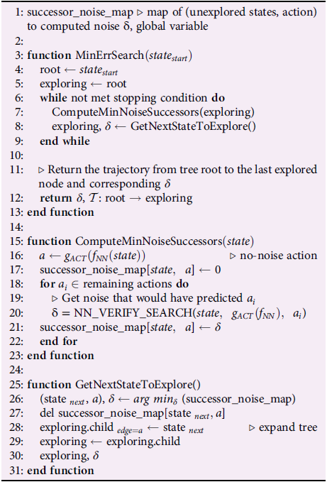
Algorithm 1. Exact Search Algorithm
Algorithm 1 describes three functions: (i) the outer-loop method that starts and terminates the search (MinErrSearch), (ii) the computation of noisy states using an open-loop neural network verification solver (ComputeMinNoiseSuccessor), and (iii) a method for determining the next node to explore (GetNextStateToExplore). We keep track of noisy states and corresponding trajectories ${\cal T}$
by representing each tree node as an object that stores both the original and noisy states. The initial state (
${\cal T}$
by representing each tree node as an object that stores both the original and noisy states. The initial state ( $stat{e_{start}}$
) is the root of the tree. For simplicity of the presentation of Algorithm 1, we omit the explicit storage and tracking of the noisy states. Nodes are explored in order of the increasing observation noise. The search concludes when a leaf node has been found such that its trajectory (the path from the root) violates the specification. In effect, we continue building out a trajectory until the noise needed to expand it further exceeds that of any other possible trajectory, and the search concludes when a path has been found to violate a safety property. The computeMinNoiseSuccessors function computes the smallest deviation to a state that would cause an incorrect target action to be predicted. This leverages open-loop neural network verification methods, which return a noisy state (the counterexample) for a fixed amount of noise. The NN_VERIFY_SEARCH function computes the smallest noise threshold that would cause a change in action. This is done through multiple calls to an open-loop neural network verification algorithm (Brix et al., Reference Brix, Müller, Bak, Johnson and Liu2023), where the exact noise threshold needed to cause a change in action is computed using a binary search. The minimum trajectory noise therefore depends on the tolerance of the binary search. Some nodes are reachable with no noise (these represent the natural behavior of the system); however, with no upper bound on added noise, all paths could be made feasible.
$stat{e_{start}}$
) is the root of the tree. For simplicity of the presentation of Algorithm 1, we omit the explicit storage and tracking of the noisy states. Nodes are explored in order of the increasing observation noise. The search concludes when a leaf node has been found such that its trajectory (the path from the root) violates the specification. In effect, we continue building out a trajectory until the noise needed to expand it further exceeds that of any other possible trajectory, and the search concludes when a path has been found to violate a safety property. The computeMinNoiseSuccessors function computes the smallest deviation to a state that would cause an incorrect target action to be predicted. This leverages open-loop neural network verification methods, which return a noisy state (the counterexample) for a fixed amount of noise. The NN_VERIFY_SEARCH function computes the smallest noise threshold that would cause a change in action. This is done through multiple calls to an open-loop neural network verification algorithm (Brix et al., Reference Brix, Müller, Bak, Johnson and Liu2023), where the exact noise threshold needed to cause a change in action is computed using a binary search. The minimum trajectory noise therefore depends on the tolerance of the binary search. Some nodes are reachable with no noise (these represent the natural behavior of the system); however, with no upper bound on added noise, all paths could be made feasible.
Algorithm 1 is guaranteed to return the trajectory associated with the least required noise, given a bound on the length of the simulation. Additionally, terminating the search at any time will yield a lower bound on the noise required to generate an unsafe trajectory; this is a certification that the system is robust to perturbations under this bound.
All the zero-noise paths are initially explored before we explore any node that requires some non-zero noise. While simulating a well-trained agent forward in time, the expansion of zero-noise paths will not terminate unless provided a maximum simulation duration (equivalently: maximum depth of the tree). Importantly, limiting the tree depth guarantees that the search will conclude and that an unsafe trajectory will be found, assuming one exists. Once all safe paths have been exhausted, the search will consider higher magnitudes of noise; given sufficient noise and a finite trajectory length, finding a path that meets the unsafe specification will always be possible.
A simplified (two control actions) illustration of the tree-building process for an aircraft collision avoidance problem is presented in Figure 2. The search is performed forward in time. The root of the tree represents a specific collision state, and the node numbers correspond to the exploration order determined by Algorithm 1. Initially, the zero-noise successors in nodes $\# 1$
and
$\# 1$
and $\# 2$
are explored. As no other 0-noise successors exist, the global noise threshold is raised, and ComputeMinNoiseSuccessors identifies the smallest magnitude of sensor noise that would reveal each potential child node. Next, node
$\# 2$
are explored. As no other 0-noise successors exist, the global noise threshold is raised, and ComputeMinNoiseSuccessors identifies the smallest magnitude of sensor noise that would reveal each potential child node. Next, node $\# 3$
is explored, since the
$\# 3$
is explored, since the $0.4{\rm{\% }}$
noise needed to actualize it is the least among potential successors revealed in the previous step. The process continues until a valid start state is found, for which we used the condition that two clear-of-conflict commands would be issued in a row. If we assume that Node
$0.4{\rm{\% }}$
noise needed to actualize it is the least among potential successors revealed in the previous step. The process continues until a valid start state is found, for which we used the condition that two clear-of-conflict commands would be issued in a row. If we assume that Node $\# 5$
is a safe state, then the trajectory of Nodes
$\# 5$
is a safe state, then the trajectory of Nodes $\# 5$
,
$\# 5$
, $\# 4$
,
$\# 4$
, $\# 1$
and the Collision State is the minimum-noise trajectory that would terminate in the given collision. No trajectory without at least 0.4% observation noise would begin in a safe state and terminate in that collision.
$\# 1$
and the Collision State is the minimum-noise trajectory that would terminate in the given collision. No trajectory without at least 0.4% observation noise would begin in a safe state and terminate in that collision.

Figure 2. Illustration of a tree generated by Algorithm 1.
Mode 2: From a final state, backward in time
The same search tree can be constructed from an initial state ${x_{init}}$
that represents a given last, unsafe, state in a trajectory. In this case, we construct a tree of state predecessors backward in time, until one is found that exists in a set of safe states. The structure of Algorithm 1 remains the same; whereas we previously enumerated potential state successors, we now enumerate potential state predecessors. Lines 16 and 18 in the function ComputeMinNoiseSuccessors instead refer to the actions that would have caused the agent to end in the given state. For both modes, we begin with
${x_{init}}$
that represents a given last, unsafe, state in a trajectory. In this case, we construct a tree of state predecessors backward in time, until one is found that exists in a set of safe states. The structure of Algorithm 1 remains the same; whereas we previously enumerated potential state successors, we now enumerate potential state predecessors. Lines 16 and 18 in the function ComputeMinNoiseSuccessors instead refer to the actions that would have caused the agent to end in the given state. For both modes, we begin with ${x_{init}}$
: one state in a given set, and search for the other end of its trajectory in the opposite set.
${x_{init}}$
: one state in a given set, and search for the other end of its trajectory in the opposite set.
Theorem 1. Algorithm 1 finds the trajectory that reaches the given collision state with the minimum sensor noise.
Proof. Let ${\cal T}$
be the unsafe trajectory returned by the search algorithm, given an unsafe end state
${\cal T}$
be the unsafe trajectory returned by the search algorithm, given an unsafe end state ${\cal S}$
. Let
${\cal S}$
. Let $er{r_{\cal T}}$
refer to the noise associated with
$er{r_{\cal T}}$
refer to the noise associated with ${\cal T}$
, or the maximum observation noise across all nodes in
${\cal T}$
, or the maximum observation noise across all nodes in ${\cal T}$
, and let
${\cal T}$
, and let ${n_{\cal T}}$
refer to the node at which
${n_{\cal T}}$
refer to the node at which $er{r_{\cal T}}$
is observed. We proceed by contradiction. Assume the returned trajectory
$er{r_{\cal T}}$
is observed. We proceed by contradiction. Assume the returned trajectory ${\cal T}$
is not the minimum-noise trajectory so that there exists another trajectory
${\cal T}$
is not the minimum-noise trajectory so that there exists another trajectory ${{\cal T}_2}$
that leads to
${{\cal T}_2}$
that leads to ${\cal S}$
with noisy
${\cal S}$
with noisy $er{r_{{{\cal T}_2}}}$
, where
$er{r_{{{\cal T}_2}}}$
, where $er{r_{{{\cal T}_2}}} \lt er{r_{\cal T}}$
. Let
$er{r_{{{\cal T}_2}}} \lt er{r_{\cal T}}$
. Let $er{r_{{{\cal T}_2}}}$
be associated with node
$er{r_{{{\cal T}_2}}}$
be associated with node ${n_{{{\cal T}_2}}}$
. Every node corresponding to trajectory
${n_{{{\cal T}_2}}}$
. Every node corresponding to trajectory ${{\cal T}_2}$
has an observation noise less than or equal to
${{\cal T}_2}$
has an observation noise less than or equal to $er{r_{{{\cal T}_2}}}$
. Since
$er{r_{{{\cal T}_2}}}$
. Since $er{r_{{{\cal T}_2}}} \lt er{r_{\cal T}}$
, every node corresponding to
$er{r_{{{\cal T}_2}}} \lt er{r_{\cal T}}$
, every node corresponding to ${{\cal T}_2}$
has an observation noise strictly less than
${{\cal T}_2}$
has an observation noise strictly less than $er{r_{\cal T}}$
. However, GetNextNodeToExplore returns the node with the least-noise child at every iteration of the search so that all nodes in
$er{r_{\cal T}}$
. However, GetNextNodeToExplore returns the node with the least-noise child at every iteration of the search so that all nodes in ${{\cal T}_2}$
must have been explored before node
${{\cal T}_2}$
must have been explored before node ${n_{\cal T}}$
is explored. This then is a contradiction, because if
${n_{\cal T}}$
is explored. This then is a contradiction, because if ${{\cal T}_2}$
was an unsafe trajectory returned by GetNextNodeToExplore, then the algorithm would have terminated and MinErrSearch would have returned
${{\cal T}_2}$
was an unsafe trajectory returned by GetNextNodeToExplore, then the algorithm would have terminated and MinErrSearch would have returned ${{\cal T}_2}$
.
${{\cal T}_2}$
.
Problem 2: Minimum noise from an initial set
The MinErrSearch algorithm yields a trajectory that begins from a given initial state ${x_0}$
. To determine the initial state associated with the global minimum-noise trajectory, we wrap calls to the function in an outer Bayesian optimization loop. The constructed Gaussian Process returns minimum-noise predictions in the form of a univariate normal distribution. We used the probability of expected improvement as the acquisition function, the normal CDF of the z-score for the minimum found value, with an added
${x_0}$
. To determine the initial state associated with the global minimum-noise trajectory, we wrap calls to the function in an outer Bayesian optimization loop. The constructed Gaussian Process returns minimum-noise predictions in the form of a univariate normal distribution. We used the probability of expected improvement as the acquisition function, the normal CDF of the z-score for the minimum found value, with an added $\varepsilon $
constant to add an exploration factor
$\varepsilon $
constant to add an exploration factor ${\rm{\Phi }}\left( {{{y{\rm{'}} - {\mu _k}\left( x \right) - \varepsilon )} \over {{\sigma _k}\left( x \right)}}} \right)$
(Brochu et al., Reference Brochu, Cora and de Freitas2010). This function favors more of an exploitation strategy if
${\rm{\Phi }}\left( {{{y{\rm{'}} - {\mu _k}\left( x \right) - \varepsilon )} \over {{\sigma _k}\left( x \right)}}} \right)$
(Brochu et al., Reference Brochu, Cora and de Freitas2010). This function favors more of an exploitation strategy if $\varepsilon $
is 0; we set
$\varepsilon $
is 0; we set $\varepsilon $
empirically.
$\varepsilon $
empirically.
Evaluation
Environments
We evaluate our approach on four systems presented in Figure 3: two benchmarks from the Open AI reinforcement learning Gym and two aerospace tasks.

Figure 3. Environments. (a): ACAS Xu from Owen et al. (Reference Owen, Panken, Moss, Alvarez and Leeper2019), (b): Dubins Rejoin from Ravaioli et al. (Reference Ravaioli, Cunningham, McCarroll, Gangal, Dunlap and Hobbs2022), (c): Cart Pole from Brockman et al. (Reference Brockman, Cheung, Pettersson, Schneider, Schulman, Tang and Zaremba2016), (d): Lunar Lander from Brockman et al. (Reference Brockman, Cheung, Pettersson, Schneider, Schulman, Tang and Zaremba2016).
These environments were chosen to demonstrate the flexibility of the tool: evaluations include runs that were performed both forward and backward on systems of varied complexity and with varied input and output dimensions. The Dubins Rejoin system was originally designed for continuous output control: we trained a discretized version for use with our tool. The ACAS Xu networks were not trained via reinforcement learning; the networks were trained to mimic a lookup table (Julian et al., Reference Julian, Lopez, Brush, Owen and Kochenderfer2016). The OpenAI benchmarks were trained with the Stable Baselines framework (default parameters from the Stable Baselines Zoo) (Raffin et al., Reference Raffin, Hill, Gleave, Kanervisto, Ernestus and Dormann2021) and the Rejoin network with the authors’ implementation. More details about the set of starting states, STL safety violations, and other training information are included in Table 1. For the aircraft collision and Lunar Lander environments, we only explore noise in the position measurements (x, y, and headings); velocities are fixed throughout all simulations. The Dubins Rejoin state observations are represented in relative terms among the lead, rejoin region, and wingman.
Table 1. Descriptions of environments used for evaluation

Neural network verification
We use the neural network verification tool nnenum to compute the closest counterexample for a given observation and target output command. The distance from the original observation and the counterexample corresponds to the least amount of noise $\rho $
that would cause the system to behave erroneously.
$\rho $
that would cause the system to behave erroneously.
The nnenum tool uses linear star sets (Duggirala and Viswanathan, Reference Duggirala and Viswanathan2016) to compute possible outputs of a neural network given constructed sets of inputs. As inputs are propagated through a network, sets are split whenever multiple output predictions (advisories) are possible. When verification is impossible, the tool yields a counterexample ( $x$
where
$x$
where $x \in {\mathbb{X}},{f_{NN}}(x) = y$
and
$x \in {\mathbb{X}},{f_{NN}}(x) = y$
and $y \in \mathbb{U}$
). Our approach relies on these counterexamples to calculate unsafe trajectories.
$y \in \mathbb{U}$
). Our approach relies on these counterexamples to calculate unsafe trajectories.
The tool takes in an observation, a target output command, and a threshold for noise (box constraints) around the observation to search within. Because the exact noise threshold for each case is unknown to us in advance, we make multiple calls to nnenum within a binary search to pinpoint the lowest noise threshold that would yield a successful counterexample. This noise threshold corresponds to the least amount of noise $\rho $
, and the counterexample corresponds to the adversarial observation of the noisy trajectory. We used a binary search tolerance of 1
$\rho $
, and the counterexample corresponds to the adversarial observation of the noisy trajectory. We used a binary search tolerance of 1 ${e^{ - 4}}$
(0.01%) of the maximum range for all experiments.
${e^{ - 4}}$
(0.01%) of the maximum range for all experiments.
In principle, any similar verification tool could be used for our approach (Bak et al., Reference Bak, Liu and Johnson2021). Tools that do not return counterexamples could still be used within our method to compute minimum magnitudes of tolerated noise; however, counterexamples are needed for returning the exact sequence of noisy observations.
Simulation direction and trajectory length
Our algorithm for Problem 1 was introduced for both forward and backward simulations in time. For efficiency, the direction chosen should depend on the relative sizes of the safe and unsafe states. For example, the set of possible initial states for the ACAS Xu system is much larger than the set of collision states, so we choose to perform Bayesian optimization over the unsafe collision states and explore trajectories backward in time. One advantage of conducting the search beginning with terminal unsafe states, is that a maximum simulation length is not required. With sufficient noise, the search is guaranteed to reach a safe state, yielding a trajectory that begins safely yet terminates in the supplied unsafe state. In contrast, if simulating forward from a safe state using a well-trained network, the system might never reach an unsafe state when following a 0-noise path along the tree. For this reason, we acknowledge limitations around scalability and, in practice, limit the length of the trajectories explored. This constraint guarantees that we will explore unsafe trajectories within a reasonable time, similar to limiting the length of the simulation while training the agent.
The Cart Pole and Lunar Lander evaluations were performed forward in time, and the trajectory lengths were capped at 15 timesteps. While the noise threshold returned by our approach for these systems serves as an upper bound on the true minimum, it still offers certainty that the system is provably safe within a given time horizon. Moreover, existing techniques for identifying stealthy adversarial perturbations similarly focus on a specific, vulnerable time horizon. Comparisons with these state-of-art techniques are included in the Evaluation section.
Results
Table 2 presents the least-noisy trajectory observed from uniform samples of initial states. Results are filtered to include only initial states that would have been safe without interference. Multiple minimal-noise trajectories were generated from an independent MinErrSearch (Problem 1). Each row describes the unsafe trajectory associated with the least magnitude of noise across all trials. The last two columns contextualize this noise in terms of the initial state and maximum deviation in real units.
Table 2. Global minimum-noise trajectories from random and uniform samples

ACAS Xu
Figure 4 presents unsafe trajectories found by our approach on the ACAS Xu system. Steps along each trajectory that could only be realized with sensor noise are shown in red, whereas steps without noise are shown in black. Gaps in this figure indicate regions of starting states that are safe from future collision with under 1% noise. For instance, no trajectory that terminates in a collision that we sampled begins in a tail-chasing scenario (region at the bottom half of the plot).

Figure 4. Minimum-noise trajectories leading up to each collision point around the intruder aircraft (minimum for each position across all headings).
Interestingly, these trajectories are not symmetric around the intruder: this is consistent with observations that the response of the aircraft at single time steps is not entirely symmetric (Katz et al., Reference Katz, Barrett, Dill, Julian and Kochenderfer2017a).
The noise associated with each trajectory is displayed in Figure 5 along with its ending position and heading at collision. Darker cells in the heatmap correspond to smaller minimum-noise trajectories and represent more vulnerable portions of the collision surface. Cells with a white border emphasize the least-noise heading per row. The green cell indicates the smallest magnitude of noise, which quantifies the system’s robustness: no smaller amount of noise will lead the aircraft into collision.

Figure 5. Noise required to end in collisions specified by position and heading. Each cell represents the least magnitude of noise required to form a trajectory that ends at the corresponding collision position/heading. The least value per row is highlighted in white; the least noise overall is in green.
Dubins Rejoin
Results from 16 runs of the Dubins Rejoin environment are presented in Figure 6. We sampled safe starting points along the bottom half of a lead radius of 500 ft ( $\pi $
to
$\pi $
to $2\pi $
rad): properly trained rejoin networks should control the wingman to stay within the rejoin region and avoid flying closer to the lead. The inner circle in Figure 6 represents the collision radius of 150 ft. The color of each point represents the least amount of noise required to force the lead to cross the collision radius. The least noise observed across the start space was 7.1% of the input ranges, which translates to under 100 ft of uncertainty in the sensed positions (smaller than the length of the aircraft). The trajectories on either side of
$2\pi $
rad): properly trained rejoin networks should control the wingman to stay within the rejoin region and avoid flying closer to the lead. The inner circle in Figure 6 represents the collision radius of 150 ft. The color of each point represents the least amount of noise required to force the lead to cross the collision radius. The least noise observed across the start space was 7.1% of the input ranges, which translates to under 100 ft of uncertainty in the sensed positions (smaller than the length of the aircraft). The trajectories on either side of ${3\pi }\over{2}$
rad are not completely symmetrical, similar to those from the ACAS Xu results. Again, similarly, the states closer to a tail-chasing collision are the most robust. This is likely because these states represent situations where the wingman can avoid collision without turning sharply.
${3\pi }\over{2}$
rad are not completely symmetrical, similar to those from the ACAS Xu results. Again, similarly, the states closer to a tail-chasing collision are the most robust. This is likely because these states represent situations where the wingman can avoid collision without turning sharply.

Figure 6. Least noise required to end in a collision starting from uniform initial states around the lead. The least across all runs is indicated by the arrow. The initial states plotted are within the rejoin region; the collision radius is shown by the inner circle.
Relevance to continuous-control systems: The Dubins Rejoin system can be implemented for both continuous or discrete action spaces. We investigated the extent to which findings from our approach can generalize from the discretized version to the original continuous-control version by applying the perturbed set of noisy observations to the original system. While we observed that the minimum separation distance between the two aircraft did approach the collision radius, none of the trials ended in collision. This is likely due to the size of the bins and the resulting difference in network controllers: we discretized the action space into 4 points for both the rudder and throttle actuators so that each node in the search tree had a maximum of 16 children. Smaller bins would likely result in similar controllers but with runtime tradeoffs.
Cart Pole
We evaluate on the benchmark Cart Pole problem to illustrate yet another use of our approach: understanding how clean and adversarial trajectories tend to differ. Figure 7 shows differences between clean and adversarial trajectories originating from each initial safe state; trajectories in red are those that would lead to a crash from the initial point with the least amount of sensor noise. The least-noise trajectories tended to push the cart right (higher position values in the “Cart position” subplot), causing the pole to tip counter-clockwise (lower angle values in the “Pole Angle” subplot). This illustrates a bias in the trained control network: components involved in controlling the cart right are more vulnerable to small amounts of noise than components involved in the left control. Moreover, we see that adversarial trajectories tend to have higher linear and angle velocities across all steps.

Figure 7. Cart Pole clean and adversarial states over min-noise trajectories. Blue lines represent the original (no-noise) trajectories from each initial state, and red lines represent the corresponding adversarial trajectories (The X-axis is time). The unsafe paths tend to force the cart right and pole counter-clockwise, which suggests uneven vulnerabilities in the control network. The unsafe paths additionally resulted in higher magnitude cart and pole velocities.
Lunar Lander
The Lunar Lander experiments were initialized from two separate regions near each landing pad pole, and trajectories were capped at a maximum depth of 30 steps from the start. Our method revealed many starting states that ended in a crash naturally; this approach provides a quantifiable metric for assessing the quality of a network. However, our approach also revealed the existence of trajectories that would have been safe without noise. These trajectories reveal vulnerabilities in a network that would have otherwise handled the case appropriately. Similar to the cartpole setting, some adversarial trajectories were also associated with higher linear and angular velocities: the landers make contact with the moon faster than in the clean settings. We reserve plots similar to Figures 5 and 7 for the appendix.
Properties of unsafe trajectories
Positions and frequency of required noisy readings
Intuitively, as an agent approaches an unsafe state, the control network should be more robust to sensor noise than it might have been farther away. However, we observed that the simulation step associated with maximum sensor noise over unsafe trajectories was not always close to the near-collision state. The ACAS Xu and Cart Pole systems did satisfy expectations: the largest noise along a trajectory tended to be closer to the collision.
However, the Dubins Rejoin and Lunar Lander distributions are less intuitive: the most critical points for noise injection were often at the start of a trajectory.
We can further analyze whether noisy observations were required across most trajectory steps or if the safety violation resulted from just a few noisy readings. While the unsafe trajectories generally require small amounts of noise ( $ \lt 1\% $
of the range of each input), a large proportion of steps in each trajectory required some noise to keep the agents along an unsafe path. For ACAS Xu and Dubins Rejoin, most trajectories needed over
$ \lt 1\% $
of the range of each input), a large proportion of steps in each trajectory required some noise to keep the agents along an unsafe path. For ACAS Xu and Dubins Rejoin, most trajectories needed over $75{\rm{\% }}$
of steps to have noise for the system to reach an unsafe state. On the other hand, most trajectories from the Cart Pole and Lunar Lander environments only required noise under half the time. Nevertheless, no unsafe trajectories were realized across all experiments and environments with noise at just 1 timestep.
$75{\rm{\% }}$
of steps to have noise for the system to reach an unsafe state. On the other hand, most trajectories from the Cart Pole and Lunar Lander environments only required noise under half the time. Nevertheless, no unsafe trajectories were realized across all experiments and environments with noise at just 1 timestep.
Overall, we find that minimum-noise unsafe trajectories are generally the result of consistent noisy readings, mostly during simulation steps closer to an unsafe state. Additional plots to support these claims are included in the appendix.
Ablation experiments: Per-variable noise
We can use our method to further investigate how the control networks are vulnerable to noise along specific input dimensions. We performed ablation experiments with the ACAS Xu system as a case study on the three inputs: ${\rm{\rho }},{\rm{\theta }},{\rm{\psi }}$
; full details are included in Table 3.
${\rm{\rho }},{\rm{\theta }},{\rm{\psi }}$
; full details are included in Table 3.
Table 3. Results from a set of ablation (masking) experiments for ACAS Xu. As expected, the noise required for the least-noise unsafe trajectories decreases as more variables are allowed uncertainty. Moreover, we observe that the variable $\theta $
is most vulnerable to noise: it consistently takes a smaller magnitude of noise across all variables when
$\theta $
is most vulnerable to noise: it consistently takes a smaller magnitude of noise across all variables when $\theta $
is included. Of all experiments when just one variable is allowed uncertainty, the one where
$\theta $
is included. Of all experiments when just one variable is allowed uncertainty, the one where $\theta $
is noisy requires the least noise (note that all values are percentages of the allowed range for each variable, normalized to
$\theta $
is noisy requires the least noise (note that all values are percentages of the allowed range for each variable, normalized to $\left[ { - 1.0,{\rm{\;}}1.0} \right]$
)
$\left[ { - 1.0,{\rm{\;}}1.0} \right]$
)

We observe that variable ${\rm{\theta }}$
is most sensitive – an unsafe trajectory was found with just
${\rm{\theta }}$
is most sensitive – an unsafe trajectory was found with just $4.96$
of noise in
$4.96$
of noise in ${\rm{\theta }}$
(
${\rm{\theta }}$
( $1.3785{\rm{\% }}$
of its range). Fixing
$1.3785{\rm{\% }}$
of its range). Fixing ${\rm{\theta }}$
yields unsafe trajectories with much higher noise. A similar analysis could be performed on other systems to reveal vulnerabilities in certain input dimensions. These results could help prioritize how to safeguard against sensor spoofing attacks.
${\rm{\theta }}$
yields unsafe trajectories with much higher noise. A similar analysis could be performed on other systems to reveal vulnerabilities in certain input dimensions. These results could help prioritize how to safeguard against sensor spoofing attacks.
Effectiveness of Bayesian optimization
For environments whose initial safe states span a large range, we show that the Bayesian optimization proposed in Problem 2 adequately estimates the most vulnerable starting state. We present a case study of this optimization for the ACAS Xu system due to its large initial state space (all points on a circle at 500 ft around the intruder aircraft). Random or uniform sampling for Cart Pole and Lunar Lander is sufficient as their initial starting regions are small. The ACAS Xu system is similar to Dubins Rejoin; we focus this work on just the former to illustrate its use and avoid redundancy.
We compared the least noise found via random sampling with that found via Bayesian Optimization over the start-space domain for the same number of calls to MinErrSearch. Figure 8 shows how the number of calls needed scales when approaching the global minimum of $0.63{\rm{\% }}$
. Random sampling needs an average of more than
$0.63{\rm{\% }}$
. Random sampling needs an average of more than $200$
iterations, while Bayesian Optimization only needs
$200$
iterations, while Bayesian Optimization only needs $\sim$
110 to approach the global minimum.
$\sim$
110 to approach the global minimum.

Figure 8. Comparison of Bayesian Optimization and Random Sampling for uniform grid points for ACAS Xu. MinErrSearch iterations are run until a noise limit is reached. Both techniques perform similarly until the global minimum is approached, beyond which Bayesian methods perform significantly better.
The exact global minimum was not found consistently with Bayesian Optimization because of the location of its corresponding state: the Matern kernel function makes assumptions of smoothness for the objective function it mimics. We confirmed that the location of the exact global minimum is located in a region with discontinuous values, making exploitation later in the search ineffective as the valley is overlooked. Instead, Bayesian optimization identified the state with the second smallest uniformly-sampled point ( $0.65{\rm{\% }}$
), which is a useful upper bound on the robustness of the system. While we demonstrated this outer-loop technique on just the ACAS Xu system, we expect similar results for other systems.
$0.65{\rm{\% }}$
), which is a useful upper bound on the robustness of the system. While we demonstrated this outer-loop technique on just the ACAS Xu system, we expect similar results for other systems.
Comparisons with reinforcement learning adversarial attack methods
While our approach is the first to guarantee the smallest magnitude of noise that can cause a system to fail, we note that a parallel body of work addresses adversarial testing of agents trained via Reinforcement Learning. These works tend to focus on developing attack strategies that empirically cause the system to fail, given various limitations, by relying on training models to forecast future states and leverage probabilistic machine learning approaches that generate counterexamples at each time step.
Early works by Lin et al. (Reference Lin, Hong, Liao, Shih, Liu and Sun2017) and Sun et al. (Reference Sun, Zhang, Xie, Ma, Zheng, Chen and Liu2020) focused on developing attack strategies that minimize the number of perturbed time steps throughout a trajectory. Lin et al.’s “Strategic Attack” proposes using a heuristic to inform when to attack. Their timing heuristic is based on the preference of an agent taking one action over another, and the attack uses a Projected Gradient Descent method (Madry et al., Reference Madry, Makelov, Schmidt, Tsipras and Vladu2017) to perturb the observations when the metric exceeds a tuned hyperparameter. Sun et al.’s “Critical Point Attack” (2020) expands on this by using a planning model to seek the most critical set of consecutive timesteps to attack. More recently, Zhang et al. (Reference Zhang, Chen, Boning and Hsieh2021) developed an attack method that learns an adversarial agent that perturbs state observations to minimize the reward of its environment. They frame the adversarial agent as a Markov Decision Process (MDP) that uses the negative of the reward defined by the nominal training process to train a new neural network that approximates this adversary. The new network generates the sequence of adversarial perturbations for a supplied trajectory length and noise cap; we refer to this strategy as the “MDP Attack.”
Although the intended uses of our approach and the mentioned attack strategies differ, we present these comparisons to highlight how our certified approach can not only identify more optimal attacks but also serve as a baseline for evaluating the optimality of such attack strategies. We focus on the three aforementioned strategies because they have publicly released their code and cover common strategies (thresholded heuristic, planning method, and training an adversarial agent). We used public-source implementations of Strategic Attack, Critical Point Attack, MDP Attack on GitHub. Footnote 1,Footnote 2 Figures 9 and 10 present our results on the CartPole system.

Figure 9. Attack strength v success rate, over 50 trials. The MDP (Zhang et al., Reference Zhang, Chen, Boning and Hsieh2021), Critical Point (Sun et al., Reference Sun, Zhang, Xie, Ma, Zheng, Chen and Liu2020), and Strategic (lin_tactics_2019) Attacks require a set noise percentage; as that noise increases, we observe the chance of success increasing. The first percentage at which we observe a successful attack is 1.65%, 13.2%, and 14.7%, respectively, compared with 1.6% from our method for a guaranteed 100% success, noise needs to reach 2.5%, 18.5%, and 23.9% respectively. Increasing the allowed noise percentage does not change the minimum-error trajectories we obtain with our method.
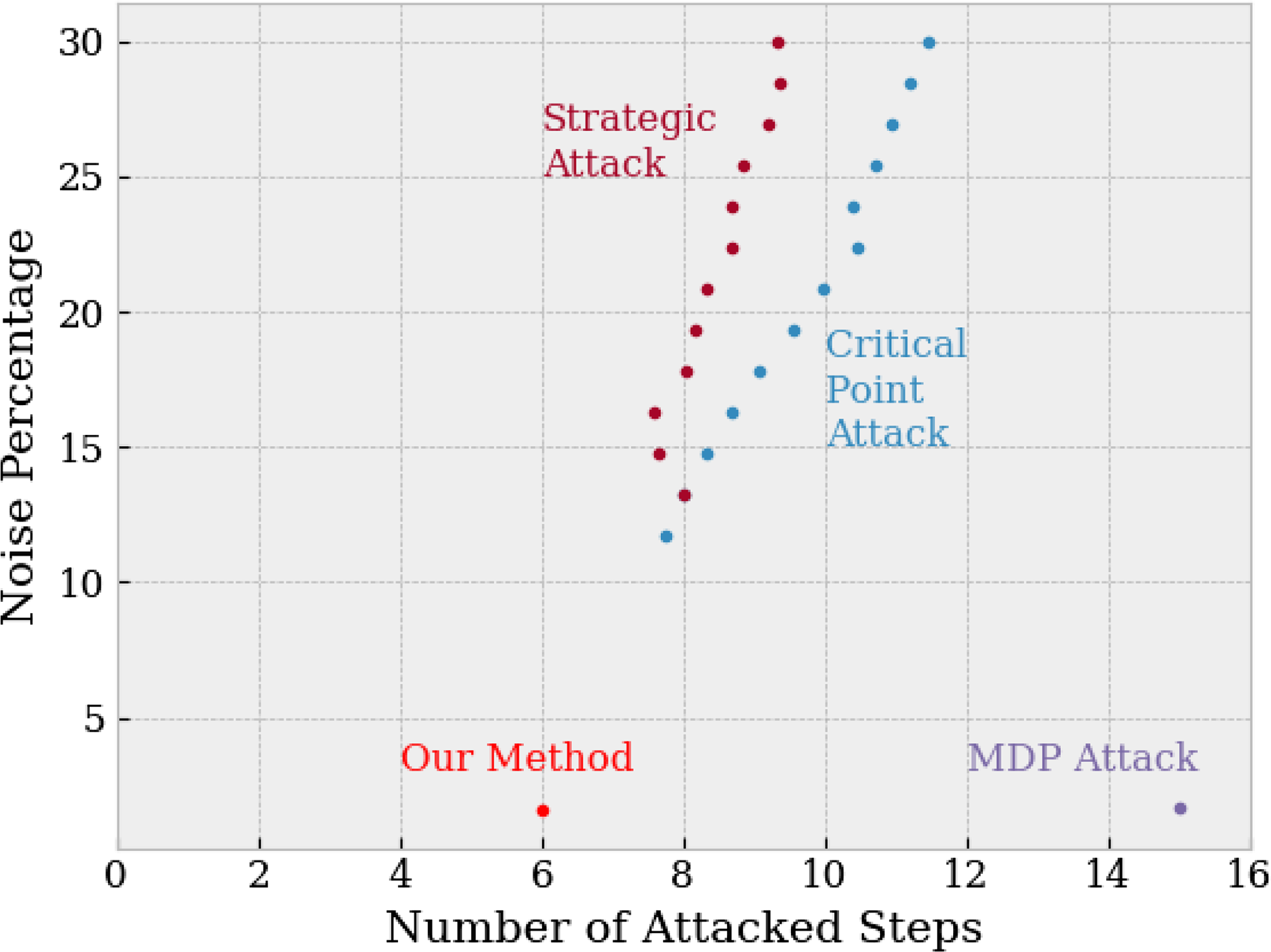
Figure 10. Comparison among the noise percentage associated with the number of attacked steps. The simpler Strategic and Critical Point strategies generally required about 8 attacked steps. The MDP Attack found successful unsafe trajectories at 1.65%, close to the 1.6% minimal noise found by our method. However, the strategy attacks all steps within the specified trajectory length, whereas we identified trajectories with as few as 6 attacked steps.
First, we compare our approach against these recent methods to examine whether other methods identify the certified, smallest amount of noise found by our approach to cause a system failure. Empirical methods are not guaranteed to succeed; therefore, we report the attack success as a rate over 50 trials for which we previously found a minimal-error trajectory of 1.6%. Figure 9 presents these results for the CartPole system. While our technique is able to find the minimum-noise trajectory at $1.6{\rm{\% }}$
(represented by a straight line), the Strategic and Critical Point attacks only succeed when the provided magnitude of noise exceeds 10%. The MDP Attack, however, comes close: the smallest noise percentage seen to generate a successful attack is
$1.6{\rm{\% }}$
(represented by a straight line), the Strategic and Critical Point attacks only succeed when the provided magnitude of noise exceeds 10%. The MDP Attack, however, comes close: the smallest noise percentage seen to generate a successful attack is $1.65{\rm{\% }}$
(notably not seen at 1.6%). However, guaranteed failure (attack success at 100%) was only observed when the noise tolerance reached
$1.65{\rm{\% }}$
(notably not seen at 1.6%). However, guaranteed failure (attack success at 100%) was only observed when the noise tolerance reached $2.5{\rm{\% }}$
.
$2.5{\rm{\% }}$
.
Next, as many reinforcement learning attack methods seek to reduce the number of attacked timesteps and maintain attack success, we compare the number of attacked steps and required noise percentage across attack strategies. Figure 10 presents the relationship between attacked steps and noise: intuitively, as the supplied noise cap increases, the number of successfully attacked steps could increase (in order to maximize overall attack success). The Strategic and Critical Point attacks show this relationship; they were able to generate unsafe trajectories with about 8 attacked steps. The MDP Attack, similar to our own, requires planning (and potentially attacking) all steps of a trajectory of a supplied length; we limited the Cart Pole trajectories to 15 steps for comparison with our method.
Overall, the gradient-based strategies failed to find attacks as stealthy as our method and MDP. The MDP approach empirically neared the stealthiest possible attack, which was demonstrated by a comparison with our certified approach. Going forward, we believe our method can continue to be used to evaluate the robustness of RL systems and adversarial strategies, especially as this approach can evaluate networks not trained via reinforcement learning.
Related work
Existing research on the safety of neural network controllers in cyber-physical systems generally lies in three categories: (1) on the demonstration of sensor spoofing or feasible perturbations in specific environments, (2) on anomaly detection algorithms to filter noisy observations, and (3) on identifying optimal adversarial perturbations or unsafe initial conditions for an agent. Our work is most closely related to the last area of research, with a focus on formal verification.
Neural network verification seeks to prove the properties of neural networks by relating sets of inputs to all possible sets of outputs. The formal verification problem has been shown to be NP-Complete (Katz et al., Reference Katz, Barrett, Dill, Julian and Kochenderfer2017b), so contemporary work looks at efficient implementations for practical scalability of verification tools to larger networks (Bak et al., Reference Bak, Liu and Johnson2021; Liu et al., Reference Liu, Arnon, Lazarus, Strong, Barrett and Kochenderfer2019; Xiang et al., Reference Xiang, Musau, Wild, Lopez, Hamilton, Yang, Rosenfeld and Johnson2018).
Existing work on adversarial trajectories has focused on strategies to perturb a sequence of sensed states that empirically result in unsafe outcomes. Huang et al. (Reference Huang, Papernot, Goodfellow, Duan and Abbeel2017) were the first to show that neural network policies can be susceptible to adversarial attacks. The authors examined the feasibility of gradient-based attacks on policies and the transferability of examples across policies. While they showed that an adversary was able to effectively decrease accumulated rewards during an episode by attacking every frame, they did not aim to target specific actions or undesired states strategically. At the same time, Kos and Song (Reference Kos and Song2017) evaluated adversarial examples against random noise and the effectiveness of re-training control policies. Lin et al. (Reference Lin, Hong, Liao, Shih, Liu and Sun2017) improved on the Huang et al. attack with methods for selectively modifying important frames and probabilistically guiding the agent to a target state. Moreover, Sun et al. (Reference Sun, Zhang, Xie, Ma, Zheng, Chen and Liu2020) looked to prediction models to determine the least number of timesteps to attack. A more recent approach by Zhang et al. (Reference Zhang, Chen, Boning and Hsieh2021) adopts a MDP to learn the optimal adversarial attack for RL agents. This process is still empirical in nature, as it relies on the accuracy of the trained MDP model.
In contrast to these works, each trajectory that our approach generates ends in an unsafe state. Fundamentally, our approach is the first to provide certified guarantees. The data that support the findings of this study are available on request from the corresponding author.
Conclusion
Neural networks are being increasingly considered in a wide variety of systems to handle control decisions. However, the susceptibility of these networks to observation noise limits their adoption in safety-critical systems. Whereas methods like adversarial training can increase empirical robustness against such attacks, they do not offer formal guarantees.
In this paper, we proposed a method to find the minimum-noise failing trajectory for a neural network control system. Our approach is restricted to networks with discrete action spaces, and since the approach essentially constructs a tree of possible trajectories with increasing noise values, attack generation can only succeed when the number of such paths is not too large. When these restrictions are met, however, our method is able to provide a strong formal guarantee that no trajectory of smaller noise is possible from the given start state. We have applied the method to four systems in order to demonstrate its practical applicability, and were able to find situations where noise under 1% of an input range can cause these systems to fail. Our results also lay the groundwork for the design of more certifiably-robust systems. For instance, minimum-error unsafe trajectories might be used to retrain networks, after which analysis could be repeated to increase provable noise robustness.
Further, the masking experiments where we explored only attacking specific sensors revealed that some inputs could tolerate more noise than others. This knowledge could be used to prioritize deployment of safeguards against spoofing attacks or to determine where to run anomaly detection systems.
Acknowledgements
This material is based upon work supported by the Air Force Office of Scientific Research and the Office of Naval Research under award numbers FA9550-19-1-0288, FA9550-21-1-0121, FA9550-23-1-0066 and N00014-22-1-2156, as well as the Air Force Research Laboratory Innovation Pipeline Fund. Any opinions, findings, and conclusions or recommendations expressed in this material are those of the authors and do not reflect the views of the United States government, the Department of Defense, the United States Air Force or the United States Navy.
Competing interests
Multiple authors of this work have been employed by the Air Force Research Lab.
Supplementary material
To view supplementary material for this article, please visit https://doi.org/10.1017/cbp.2023.5


 Open access
Comments
No accompanying comment.