


1. Introduction
In recent years, there has been a significant amount of work on developing the lower limb powered exoskeletons to assist human motion to enhance human strength, reduce human metabolic energy cost, and rehabilitate abilities lost due to brain injuries, spinal cord injuries, and strokes [Reference Young and Ferris1–Reference Terrazas-Rodas, Rocca-Huaman, Ramírez-Amaya and Alvarez-Rodriguez3]. In the United States, it is estimated that 8.79 million people between the ages of 21 and 64 years have difficulties in lifting objects [Reference Houtenville, Brucker and Lauer4]. In addition, the exoskeletons can prevent injuries and increase human endurance for lifting tasks. Specifically, the knee joint plays a vital role in completing the transition [Reference Wretenberg and Arborelius5]. Therefore, design and control of a powered knee exoskeleton are important for lifting tasks. Moreover, experimental validation of the control of the exoskeleton in the laboratory is required before implementation.
Over the past few years, various optimization-based dynamic modeling techniques have been investigated to simulate exoskeleton–wearer interaction [Reference Bai and Rasmussen6–Reference Cho, Kim, Yi, Jung and Lee8]. In a recent study [Reference Zhou and Chen9], an integrated human-in-the-loop simulation approach was used to design and evaluate a lower limb exoskeleton. A novel two-torque compensation controller to minimize spring interaction forces and maximize assistance was virtually designed and evaluated for the lower leg exoskeleton. Running motions were used to investigate the exoskeleton effects on the wearer’s biomechanical loading conditions. In ref. [Reference Arefeen and Xiang10], a physics-based optimization formulation was proposed to find the optimal control of a powered elbow exoskeleton to aid the human–robot collaborative lifting task.
For lifting assistance, there have been a limited amounts of studies on developing both active and passive exoskeletons to assist humans in the literature [Reference Wei, Zha, Xia, Gu and Lin11–Reference Sado, Yap, Ghazilla and Ahmad19]. Wei et al. [Reference Wei, Zha, Xia, Gu and Lin11] used a semi-squat symmetric lifting model to obtain the hip joint torque and power for a lifting task. An adaptive hip active exoskeleton system was designed based on the power output curve of the hip joint during lifting. Millard et al. [Reference Millard, Sreenivasa and Mombaur14] built a 12-degrees-of-freedom (DOFs) two-dimensional (2D) human model with a 3-DOFs box and 9-DOFs motor-driven spine and hip exoskeletons. A sequential quadratic programming (SQP)-based direct optimal control approach was used to predict the human movements and the forces during the lifting to reduce the lower back injury. A powered pneumatic driven 1-DOF back exoskeleton was proposed in ref. [Reference Heo, Kim and Kim15] to assist lifting motion. It was reported that the developed prototype could mitigate lower back pain by reducing muscle activity range from 18 to 25% during lifting tasks. Sado et al. [Reference Sado, Yap, Ghazilla and Ahmad19] designed and controlled a 6-DOFs active–passive lower-body exoskeleton to maximize the human joint torques and minimize the muscular activation for squatting and walking assistance in manual material handling tasks.
Some researchers have developed only knee joint powered exoskeletons to reduce metabolic cost and muscle activities for squat lifting [Reference Zhang and Huang18–Reference Gams, Petrič, Debevec and Babič20]. Gams et al. [Reference Gams, Petrič, Debevec and Babič20] used three different controllers (gravity compensation, position, and oscillator-based) in the knee exoskeleton to compare the effects on metabolic consumption during squatting. An electromyography (EMG)-driven semi-active knee exoskeleton was designed by Wang et al. [Reference Wang, Wu, Zhang, Chen, Liu, Liu and Ma21] to reduce the muscle fatigue of the lower limb when squatting. Although the exoskeleton developed by Yu et al. [Reference Yu, Huang, Wang, Lynn, Sayd, Silivanov and Su22] was highly back-drivable and had high torque, it lacked the optimal control of the exoskeleton. Several knee-powered exoskeletons were also developed to assist human mobility tasks similar to squat lifting, such as standing up and sitting down [Reference Shepherd and Rouse23, Reference Karavas, Ajoudani, Tsagarakis, Saglia, Bicchi and Caldwell24]. Shepherd et al. [Reference Shepherd and Rouse23] proposed a novel series elastic actuated (SEA) configuration for a knee exoskeleton. The exoskeleton was able to track the desired torque using a torque sensor by employing the motor’s current as the input of torque control for sit-to-stand assistance. Karavas et al. [Reference Karavas, Ajoudani, Tsagarakis, Saglia, Bicchi and Caldwell24] developed a knee exoskeleton for standing-up and sitting-down motion assistance where a SEA was utilized to actuate the exoskeleton. In recent studies [Reference de Andrade, Fabriz Ulhoa, Fragoso Dias, Filho and Vimieiro25–Reference Wu, Yang, Xia and Wang28], there has been a significant improvement in the development of powered knee and hip exoskeletons, particularly in terms of their design, actuation, and learning-based control, which make these devices more effective in assisting with walking and rehabilitation.
In this study, we propose a subject-specific optimal control strategy for powered knee exoskeletons for squat lifting tasks. The proposed work uses inverse dynamics optimization to predict the human-exoskeleton symmetric lifting motion and optimal assistive torque. An SQP algorithm in sparse nonlinear optimizer (SNOPT) is used to solve the lifting optimization problem [Reference Gill, Murray and Saunders29]. The predicted optimal results are used in the human-exoskeleton lifting control strategy. A new exoskeleton control strategy is implemented in the experimental setup to provide real-time optimal assistance to the human knee joint during lifting. Comparisons are carried out between the simulation and experimental data.
The contents are organized as follows: the human-exoskeleton models are first described in Section 2, and the equations of motion (EOM) are also detailed in Section 2. The optimization formulation for the lifting problem is presented in Section 3. The detailed exoskeleton control strategy and experimental setup are discussed in Section 4. Section 5 presents the simulation results. The lifting validations with and without exoskeletons are also presented. Finally, discussion and concluding remarks are given in Section 6.
2. Human-exoskeleton model and EOM
The human-exoskeleton system consists of a human-exoskeleton model and its kinematics and dynamics. Denavit–Hartenberg (DH) representation method was used to express the kinematics of the human mechanical system [Reference Denavit and Hartenberg30].
2.1. Human-exoskeleton model
A 2D human skeletal model is considered in this work [Reference Zaman, Arefeen, Quarnstrom, Barman, Yang and Xiang31], as shown in Fig. 1(a). The human skeletal model is symmetric along the sagittal plane and has $n=10$
DOFs, including three global DOFs. In Fig. 1(b), it is illustrated that two 1-DOF powered exoskeletons are attached at the knee joints using straps for the experiment. Exoskeleton’s mass and inertia are added to the upper and lower legs mathematically. Therefore, the coupled human-exoskeleton mass and inertia of the upper and lower legs are calculated for the simulation. The human skeletal model is constructed using the robotic formulation of the DH method [Reference Denavit and Hartenberg30]. Each DOF represents relative rotation/translation of two body segments connected by a revolute/prismatic joint. For translational and rotational joints, the DOF is given in the local
$n=10$
DOFs, including three global DOFs. In Fig. 1(b), it is illustrated that two 1-DOF powered exoskeletons are attached at the knee joints using straps for the experiment. Exoskeleton’s mass and inertia are added to the upper and lower legs mathematically. Therefore, the coupled human-exoskeleton mass and inertia of the upper and lower legs are calculated for the simulation. The human skeletal model is constructed using the robotic formulation of the DH method [Reference Denavit and Hartenberg30]. Each DOF represents relative rotation/translation of two body segments connected by a revolute/prismatic joint. For translational and rotational joints, the DOF is given in the local $z$
-direction. It is noted that the global rotation joint (
$z$
-direction. It is noted that the global rotation joint ( $z_{3}$
), spine joint (
$z_{3}$
), spine joint ( $z_{4}$
), and hip joint (
$z_{4}$
), and hip joint ( $z_{7}$
) coincide at the same location. The positive directions for all the local rotation joints (
$z_{7}$
) coincide at the same location. The positive directions for all the local rotation joints ( $z_{3}\sim z_{10}$
) are clockwise in the global Y-Z plane. The two physical branches are the spine-arm branch and leg branch. Two arms are represented in the spine-arm branch by a single branch, since only 2D symmetric lifting is studied. In the leg branch, two legs are combined as a single branch, including thigh, tibia, and foot. In this study, the subject’s body segment length data are generated from the Xsens motion capture system (MVN Analyze Pro software) based on the measured height and foot length. The DH parameters for the human model are described in Table I, where L1 to L7 are the human joint link lengths.
$z_{3}\sim z_{10}$
) are clockwise in the global Y-Z plane. The two physical branches are the spine-arm branch and leg branch. Two arms are represented in the spine-arm branch by a single branch, since only 2D symmetric lifting is studied. In the leg branch, two legs are combined as a single branch, including thigh, tibia, and foot. In this study, the subject’s body segment length data are generated from the Xsens motion capture system (MVN Analyze Pro software) based on the measured height and foot length. The DH parameters for the human model are described in Table I, where L1 to L7 are the human joint link lengths.

Figure 1. (a) The 2D human skeletal model with knee exoskeleton and (b) Knee exoskeleton.
Table I. DH table for 2D human model.

2.2. Equations of motion
In this paper, the kinematics and dynamics of the human model are studied using recursive kinematics and Lagrangian dynamics, and details refer to refs. [Reference Xiang and Arefeen32, Reference Xiang, Arora, Rahmatalla and Abdel-Malek33]. The process is comprised of two parts: forward kinematics and backward dynamics. Forward kinematics transmits motion from the root to the end effectors, while backward dynamics transfers forces from the end effectors to the root. The human dynamics equation can be written as [Reference Xiang and Arefeen32, Reference Xiang, Arora, Rahmatalla and Abdel-Malek33]:
 \begin{equation}\tau _{{h_{i}}}=\mathrm{tr}\left(\frac{\partial \mathbf{A}_{\mathrm{i}}}{\partial q_{i}}\mathbf{D}_{i}\right)-\mathbf{g}^{\mathrm{T}}\frac{\partial \mathbf{A}_{i}}{\partial q_{i}}\mathbf{E}_{i}-\mathbf{f}_{k}^{\mathrm{T}}\frac{\partial \mathbf{A}_{i}}{\partial q_{i}}\mathbf{F}_{i}-\mathbf{G}_{i}^{\mathrm{T}}\mathbf{A}_{i-1}\mathbf{z}_{0}\end{equation}
where $\tau _{{h_{i}}}$
is the human torque at ith joint. On the right-hand side of Eq. (1), the first term is inertia and Coriolis torque, the second term is the torque due to gravity, the third term is the torque due to external forces, and the fourth term is the torque due to external moments:
$\tau _{{h_{i}}}$
is the human torque at ith joint. On the right-hand side of Eq. (1), the first term is inertia and Coriolis torque, the second term is the torque due to gravity, the third term is the torque due to external forces, and the fourth term is the torque due to external moments:
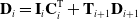 \begin{equation}\mathbf{D}_{i}=\mathbf{I}_{i}\mathbf{C}_{i}^{\mathrm{T}}+\mathbf{T}_{i+1}\mathbf{D}_{i+1}\end{equation}
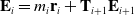 \begin{equation}\mathbf{E}_{i}=m_{i}\mathbf{r}_{i}+\mathbf{T}_{i+1}\mathbf{E}_{i+1}\end{equation}
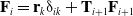 \begin{equation}\mathbf{F}_{i}=\mathbf{r}_{k}{\unicode[Arial]{x03B4}} _{ik}+\mathbf{T}_{i+1}\mathbf{F}_{i+1}\end{equation}
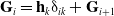 \begin{equation}\mathbf{G}_{i}=\mathbf{h}_{k}{\unicode[Arial]{x03B4}} _{ik}+\mathbf{G}_{i+1}\end{equation}
where $tr(\cdot )$
is the trace of a matrix.
$tr(\cdot )$
is the trace of a matrix. $\mathbf{A}_{i}$
,
$\mathbf{A}_{i}$
, $\mathbf{C}_{i}$
are global position and acceleration transformation matrices,
$\mathbf{C}_{i}$
are global position and acceleration transformation matrices, $\mathbf{I}_{i}$
is the inertia matrix for link i,
$\mathbf{I}_{i}$
is the inertia matrix for link i, $\mathbf{D}_{i}$
is the recursive inertia and Coriolis matrix,
$\mathbf{D}_{i}$
is the recursive inertia and Coriolis matrix, $\mathbf{E}_{i}$
is the recursive vector for gravity torque calculation,
$\mathbf{E}_{i}$
is the recursive vector for gravity torque calculation, $\mathbf{F}_{i}$
is the recursive vector for external force–torque calculation,
$\mathbf{F}_{i}$
is the recursive vector for external force–torque calculation, $\mathbf{G}_{i}$
is the recursive vector for external moment torque calculation,
$\mathbf{G}_{i}$
is the recursive vector for external moment torque calculation, $\mathbf{g}$
is the gravity vector,
$\mathbf{g}$
is the gravity vector, $m_{i}$
is the mass of link i,
$m_{i}$
is the mass of link i, $\mathbf{r}_{i}$
is the COM of link i in the
$\mathbf{r}_{i}$
is the COM of link i in the $i$
th local frame,
$i$
th local frame, $\mathbf{f}_{k}=[0 \quad f_{ky} \quad f_{kz} \quad 0]^{\mathrm{T}}$
is the external force applied on link k,
$\mathbf{f}_{k}=[0 \quad f_{ky} \quad f_{kz} \quad 0]^{\mathrm{T}}$
is the external force applied on link k, $\mathbf{r}_{k}$
is the position of the external force in the
$\mathbf{r}_{k}$
is the position of the external force in the $k$
th local frame,
$k$
th local frame, $\mathbf{h}_{k}=[h_{x} \quad 0 \quad 0\quad 0]^{\mathrm{T}}$
is the external moment applied on link k,
$\mathbf{h}_{k}=[h_{x} \quad 0 \quad 0\quad 0]^{\mathrm{T}}$
is the external moment applied on link k, $\mathbf{z}_{0}=[0 \quad 0 \quad 1 \quad 0 ]^{\mathrm{T}}$
is for a revolute joint,
$\mathbf{z}_{0}=[0 \quad 0 \quad 1 \quad 0 ]^{\mathrm{T}}$
is for a revolute joint, $\mathbf{z}_{0}=[0 \quad 0 \quad 0 \quad 0]^{\mathrm{T}}$
is for a prismatic joint, and finally,
$\mathbf{z}_{0}=[0 \quad 0 \quad 0 \quad 0]^{\mathrm{T}}$
is for a prismatic joint, and finally, ${\unicode[Arial]{x03B4}} _{ik}$
is Kronecker delta, and the starting conditions are
${\unicode[Arial]{x03B4}} _{ik}$
is Kronecker delta, and the starting conditions are $\mathbf{D}_{n+1}=[\mathbf{0}]$
and
$\mathbf{D}_{n+1}=[\mathbf{0}]$
and $\mathbf{E}_{n+1}=\mathbf{F}_{n+1}=\mathbf{G}_{n+1}=[\mathbf{0}]$
. The sensitivities to state variables are detailed in [Reference Xiang and Arefeen32, Reference Xiang, Arora, Rahmatalla and Abdel-Malek33].
$\mathbf{E}_{n+1}=\mathbf{F}_{n+1}=\mathbf{G}_{n+1}=[\mathbf{0}]$
. The sensitivities to state variables are detailed in [Reference Xiang and Arefeen32, Reference Xiang, Arora, Rahmatalla and Abdel-Malek33].
2.2.1. Exoskeleton dynamics
The electromechanical dynamics of DC motors of the exoskeletons are modeled in this study. The dynamics equations can be expressed as follows [Reference Nguyen, LaPre, Price, Umberger and Sup34]:
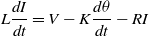 \begin{equation}L\frac{dI}{dt}=V-K\frac{d\theta }{dt}-RI\end{equation}
 \begin{equation}T_{\textit{motor}}=KI\end{equation}
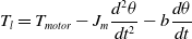 \begin{equation}T_{l}=T_{\textit{motor}}-J_{m}\frac{d^{2}\theta }{dt^{2}}-b\frac{d\theta }{dt}\end{equation}
where V, I, L, and R are the voltage input, current, inductance, and resistance, respectively. The mechanical terms $J_{m}$
, b, K, and
$J_{m}$
, b, K, and $\theta$
are the rotor moment of inertia, coefficient of viscous friction of the motor, motor torque constant, and rotor angle, respectively.
$\theta$
are the rotor moment of inertia, coefficient of viscous friction of the motor, motor torque constant, and rotor angle, respectively. $T_{\textit{motor}}$
is the motor output torque, and
$T_{\textit{motor}}$
is the motor output torque, and $T_{l}$
is the load torque of the exoskeleton. The gearbox ratios (
$T_{l}$
is the load torque of the exoskeleton. The gearbox ratios ( $GB_{r}$
) are chosen so that the devices can provide the required torque output. Here, the exoskeleton includes the motor and the gearbox. So, the output torque (
$GB_{r}$
) are chosen so that the devices can provide the required torque output. Here, the exoskeleton includes the motor and the gearbox. So, the output torque ( $\tau _{e})$
of the exoskeleton can be expressed as follows:
$\tau _{e})$
of the exoskeleton can be expressed as follows:
 \begin{equation}\tau _{e}=GB_{r}\times T_{l}\end{equation}
Furthermore, we assume that the exoskeleton’s motion aligns with human joint motion. As a result, the derivative of the rotor angle $\dot{\theta }$
and
$\dot{\theta }$
and $\ddot{\theta }$
can be expressed in terms of human joint angle derivative
$\ddot{\theta }$
can be expressed in terms of human joint angle derivative $\dot{q}$
and
$\dot{q}$
and $\ddot{q}$
with gear ratio, respectively:
$\ddot{q}$
with gear ratio, respectively:
 \begin{equation}\dot{\theta }=GB_{r}\times \dot{q}\end{equation}
 \begin{equation}\ddot{\theta }=GB_{r}\times \ddot{q}\end{equation}
where $\dot{q}$
and
$\dot{q}$
and $\ddot{q}$
are human angular velocity and acceleration for a joint, respectively.
$\ddot{q}$
are human angular velocity and acceleration for a joint, respectively.
2.2.2. Human-exoskeleton EOM
The coupled human-exoskeleton EOM and sensitivity analysis are formed using a recursive Lagrangian dynamics formulation. The overall dynamics can be expressed as follows:
 \begin{equation}\tau _{{h_{i}}}+\tau _{{e_{i}}}=\mathrm{tr}\left(\frac{\partial \mathbf{A}_{\mathrm{i}}}{\partial q_{i}}\mathbf{D}_{i}\right)-\mathbf{g}^{\mathrm{T}}\frac{\partial \mathbf{A}_{i}}{\partial q_{i}}\mathbf{E}_{i}-\mathbf{f}_{k}^{\mathrm{T}}\frac{\partial \mathbf{A}_{i}}{\partial q_{i}}\mathbf{F}_{i}-\mathbf{G}_{i}^{\mathrm{T}}\mathbf{A}_{i-1}\mathbf{z}_{0}\end{equation}
where $\tau _{{e_{i}}}$
is the exoskeleton output torque for
$\tau _{{e_{i}}}$
is the exoskeleton output torque for $i$
th joint. The ground reaction forces (GRFs) are calculated from Eq. (1) using a two-step active-and-passive algorithm in refs. [Reference Xiang and Arefeen32, Reference Xiang, Arora, Rahmatalla and Abdel-Malek33].
$i$
th joint. The ground reaction forces (GRFs) are calculated from Eq. (1) using a two-step active-and-passive algorithm in refs. [Reference Xiang and Arefeen32, Reference Xiang, Arora, Rahmatalla and Abdel-Malek33].
3. Optimization formulation
3.1. Design variables
The motor current $I(t)$
profiles and human joint profiles
$I(t)$
profiles and human joint profiles $q(t)$
are discretized using cubic B-splines [Reference Xiang, Arora, Rahmatalla, Marler, Bhatt and Abdel-Malek35]. The design variables (
$q(t)$
are discretized using cubic B-splines [Reference Xiang, Arora, Rahmatalla, Marler, Bhatt and Abdel-Malek35]. The design variables ( $\mathbf{x}$
) are human joint angle control points
$\mathbf{x}$
) are human joint angle control points $\mathbf{P}_{\textit{human}}$
and exoskeleton current control points
$\mathbf{P}_{\textit{human}}$
and exoskeleton current control points $\mathbf{P}_{\textit{current}}$
. As a result, the design variables for the human-exoskeleton motion prediction are
$\mathbf{P}_{\textit{current}}$
. As a result, the design variables for the human-exoskeleton motion prediction are $\mathbf{x}=\left[\begin{array}{c@{\quad}c} \mathbf{P}_{\textit{human}}^{\mathrm{T}} & \mathbf{P}_{\textit{current}}^{\mathrm{T}} \end{array}\right]^{\mathrm{T}}$
.
$\mathbf{x}=\left[\begin{array}{c@{\quad}c} \mathbf{P}_{\textit{human}}^{\mathrm{T}} & \mathbf{P}_{\textit{current}}^{\mathrm{T}} \end{array}\right]^{\mathrm{T}}$
.
3.2. Objective functions
The objective function is to minimize the summation of the normalized human joint torque squares [Reference Arefeen and Xiang36, Reference Arefeen and Xiang37]:
 \begin{equation}\min _{\mathbf{x}} J_{1}\left(\mathbf{x}\right)=\sum _{i=3}^{n}\int _{0}^{T}\left[\frac{\tau _{hi}(\mathbf{x})}{\left(\tau _{i}^{U}-\tau _{i}^{L}\right)}\right]^{2}dt\end{equation}
where $T$
is the specified total time for the lifting task, and
$T$
is the specified total time for the lifting task, and $\tau _{i}^{U}$
and
$\tau _{i}^{U}$
and $\tau _{i}^{L}$
are upper and lower torque limits for the
$\tau _{i}^{L}$
are upper and lower torque limits for the $i$
th joint, respectively.
$i$
th joint, respectively.
3.3. Constraints
Time-dependent constraints include (1) human joint angle limits, (2) human joint torque limits, (3) human feet contacting position, (4) box forward position, (5) collision avoidance, (6) human dynamic stability condition, and (7) exoskeleton torque limits. Time-independent constraints include (8) initial and final hand positions, (9) static conditions at the beginning and end of the motion, and (10) initial, mid-time, and final joint angles of the spine, shoulder, elbow, hip, knee, and ankle. Time-dependent constraints are calculated sequentially in the optimization process at every time discretization point. In contrast, the optimization calculates the time-independent constraints at a specific time.
(1) Human joint angle limits:
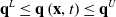 \begin{equation}\mathbf{q}^{L}\leq \mathbf{q}\left(\mathbf{x},t\right)\leq \mathbf{q}^{U}\end{equation}
where $\mathbf{q}^{L}$
and
$\mathbf{q}^{L}$
and $\mathbf{q}^{U}$
are the lower and upper joint limits for human [Reference Xiang, Zaman, Rakshit and Yang38–Reference Zaman, Xiang, Cruz and Yang41], respectively.
$\mathbf{q}^{U}$
are the lower and upper joint limits for human [Reference Xiang, Zaman, Rakshit and Yang38–Reference Zaman, Xiang, Cruz and Yang41], respectively.
(2) Human joint torque limits:
 \begin{equation}\boldsymbol{\tau }^{L}\leq \boldsymbol{\tau }\left(\mathbf{x},t\right)\leq \boldsymbol{\tau }^{U}\end{equation}
where $\boldsymbol{\tau }^{L}$
and
$\boldsymbol{\tau }^{L}$
and $\boldsymbol{\tau }^{U}$
are the lower and upper joint torque limits for human [Reference Xiang, Zaman, Rakshit and Yang38–Reference Zaman, Xiang, Cruz and Yang41], respectively.
$\boldsymbol{\tau }^{U}$
are the lower and upper joint torque limits for human [Reference Xiang, Zaman, Rakshit and Yang38–Reference Zaman, Xiang, Cruz and Yang41], respectively.
(3) Human feet contacting position:
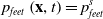 \begin{equation}p_{feet}\left(\mathbf{x},t\right)=p_{feet}^{s}\end{equation}
where $p_{feet}^{s}$
is the specified feet contact position on level ground.
$p_{feet}^{s}$
is the specified feet contact position on level ground.
(4) Box forward position:
 \begin{equation}Z_{\textit{wrist}}(\mathbf{x},t)-Z_{\textit{pelvis}}(\mathbf{x},t)\geq 0\end{equation}
where $Z_{\textit{wrist}}$
and
$Z_{\textit{wrist}}$
and $Z_{\textit{pelvis}}$
are the global Z coordinates of the human wrist and pelvis points [Reference Xiang and Arefeen32].
$Z_{\textit{pelvis}}$
are the global Z coordinates of the human wrist and pelvis points [Reference Xiang and Arefeen32].
(5) Collision avoidance:
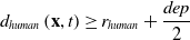 \begin{equation}d_{\textit{human}}\left(\mathbf{x},t\right)\geq r_{\textit{human}}+\frac{dep}{2}\end{equation}
where $d_{\textit{human}}$
is the calculated distance between the hand and the circle center on the body segment representing the body thickness,
$d_{\textit{human}}$
is the calculated distance between the hand and the circle center on the body segment representing the body thickness, $dep$
is the box depth, and
$dep$
is the box depth, and $r_{\textit{human}}$
is the radius of the circle filled on human limbs as shown in Fig. 2(a) [Reference Luo, Androwis, Adamovich, Nunez, Su and Zhou27]. There are seven circles on the human limb: five are on the leg (ankle, shank, knee, thigh, and hip) and two on the spine as shown in Fig. 2(b).
$r_{\textit{human}}$
is the radius of the circle filled on human limbs as shown in Fig. 2(a) [Reference Luo, Androwis, Adamovich, Nunez, Su and Zhou27]. There are seven circles on the human limb: five are on the leg (ankle, shank, knee, thigh, and hip) and two on the spine as shown in Fig. 2(b).
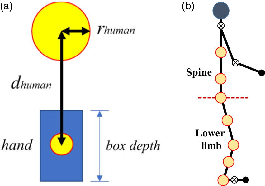
Figure 2. Collision avoidance constraint.
(6) Dynamic stability condition:
 \begin{equation}p_{\textit{human}\_ ZMP}\left(\mathbf{x},t\right)\in \mathrm{FSR}\end{equation}
where zero moment point (ZMP) position is inside the foot support region (FSR) for human [Reference Xiang and Arefeen32].
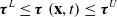
(7) Exoskeleton torque limits:
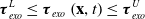 \begin{equation}\boldsymbol{\tau }_{exo}^{L}\leq \boldsymbol{\tau }_{exo}\left(\mathbf{x},t\right)\leq \boldsymbol{\tau }_{exo}^{U}\end{equation}
where $\boldsymbol{\tau }_{exo}^{L}$
is lower torque limit, and
$\boldsymbol{\tau }_{exo}^{L}$
is lower torque limit, and $\boldsymbol{\tau }_{exo}^{U}$
is the upper limit for the exoskeleton.
$\boldsymbol{\tau }_{exo}^{U}$
is the upper limit for the exoskeleton.
(8) Initial and final hand positions:
 \begin{equation}p_{\textit{human}\_ hand}\left(\mathbf{x},t\right)=p_{\textit{human}\_ hand}^{s}\left(t\right);\, t=0, T\end{equation}
where, $p_{\textit{human}\_ hand}^{s}$
is the specified hand position at initial and final times.
$p_{\textit{human}\_ hand}^{s}$
is the specified hand position at initial and final times.
(9) Initial and final static conditions:
 \begin{equation}\dot{\mathbf{q}}_{\textit{human}}\left(\mathbf{x},t\right)=\mathbf{0};\, t=0,T\end{equation}
(10) Initial, mid-time, and final joint angles for the spine, shoulder, elbow, hip, knee, and ankle:
 \begin{equation}\left| q_{i\_ \textit{human}}\left(\mathbf{x},t\right)-q_{i\_ \textit{human}}^{E}\left(t\right)\right| \leq \varepsilon ;\, t=0,\frac{T}{2},T\end{equation}
where ${\unicode[Arial]{x03B5}} =0.2$
rad, and
${\unicode[Arial]{x03B5}} =0.2$
rad, and $q_{i\_ \textit{human}}^{E}$
is the experimental joint angle for the spine, shoulder, elbow, hip, knee, and ankle joints.
$q_{i\_ \textit{human}}^{E}$
is the experimental joint angle for the spine, shoulder, elbow, hip, knee, and ankle joints.
4. Knee exoskeleton control and experiments
4.1. Control strategy
We propose a new exoskeleton control strategy which uses the offline solved optimal simulation results under the controlled environment in real time to assist human lifting. This control algorithm has two phases as shown in Fig. 3 and consists of two offline optimizations: lifting optimization and assistive torque interpolation optimization.
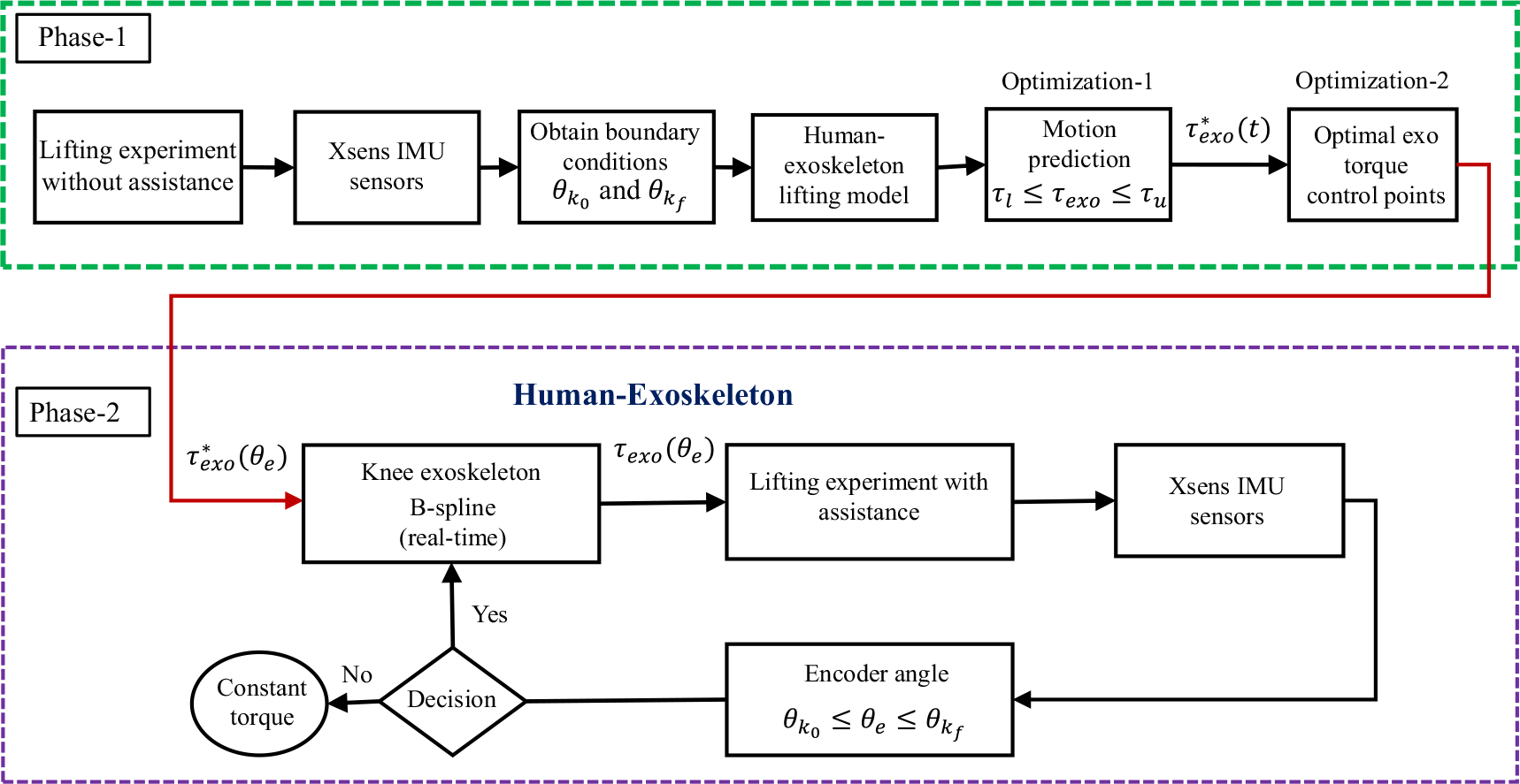
Figure 3. The diagram of the proposed lifting assistance control algorithm. Here, $\theta _{{k_{0}}}$
and
$\theta _{{k_{0}}}$
and $\theta _{{k_{f}}}$
are initial and final knee angles, respectively.
$\theta _{{k_{f}}}$
are initial and final knee angles, respectively. $\tau _{l}$
and
$\tau _{l}$
and $\tau _{u}$
are the lower and upper limits of the exoskeleton torque.
$\tau _{u}$
are the lower and upper limits of the exoskeleton torque. $\tau _{exo}^{*}(\theta _{e})$
is the optimal exoskeleton torque in joint angle domain, and
$\tau _{exo}^{*}(\theta _{e})$
is the optimal exoskeleton torque in joint angle domain, and $\tau _{exo}(\theta _{e})$
is the real exoskeleton assistive torque.
$\tau _{exo}(\theta _{e})$
is the real exoskeleton assistive torque.
In Section 2.1, we modeled a 2D human model with a knee exoskeleton. For the optimization in the first phase, an inverse dynamics optimization formulation is used to find the optimal exoskeleton torque, $\tau _{exo}^{*}(t)$
and optimal knee angle
$\tau _{exo}^{*}(t)$
and optimal knee angle $\theta _{k}^{*}(t)$
for the lifting task, as discussed in Section 3. However, for exoskeleton control, the exoskeleton reads the knee encoder angle (
$\theta _{k}^{*}(t)$
for the lifting task, as discussed in Section 3. However, for exoskeleton control, the exoskeleton reads the knee encoder angle ( $\theta _{e}$
), and outputs the exoskeleton torque, which is a function of the knee joint encoder angle
$\theta _{e}$
), and outputs the exoskeleton torque, which is a function of the knee joint encoder angle $\tau _{exo}(\theta _{e}).$
Therefore, we need to transfer the discretized optimal exoskeleton torque
$\tau _{exo}(\theta _{e}).$
Therefore, we need to transfer the discretized optimal exoskeleton torque $\tau _{exo}^{*}(t)$
obtained from the simulation in the time domain to a continuous function of the encoder angle in joint angle domain. In this study, we use a B-spline interpolation to represent
$\tau _{exo}^{*}(t)$
obtained from the simulation in the time domain to a continuous function of the encoder angle in joint angle domain. In this study, we use a B-spline interpolation to represent $\tau _{exo}(\theta _{e})$
as in Eq. (24):
$\tau _{exo}(\theta _{e})$
as in Eq. (24):
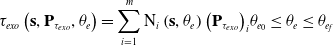 \begin{equation}\tau _{exo}\left(\mathbf{s},\mathbf{P}_{{\tau _{exo}}},\theta _{e}\right)=\sum _{i=1}^{m}\mathrm{N}_{i}\left(\mathbf{s},\theta _{e}\right){\left(\mathbf{P}_{{\tau _{exo}}}\right)}_{i} \theta _{{e_{0}}}\leq \theta _{e}\leq \theta _{{e_{f}}}\end{equation}
where s = $\left[\theta _{{e_{0}}},\ldots .\,.\,, \theta _{{e_{f}}}\right]^{\mathrm{T}}$
is the encoder angle knot vector,
$\left[\theta _{{e_{0}}},\ldots .\,.\,, \theta _{{e_{f}}}\right]^{\mathrm{T}}$
is the encoder angle knot vector, $\mathbf{P}_{{\tau _{exo}}} = \left[{(P_{{\tau _{exo}}}})_{1},\ldots \ldots, {(P_{{\tau _{exo}}}})_{m}\right]^{\mathrm{T}}$
is the exoskeleton torque control point vector, m is the number of control points,
$\mathbf{P}_{{\tau _{exo}}} = \left[{(P_{{\tau _{exo}}}})_{1},\ldots \ldots, {(P_{{\tau _{exo}}}})_{m}\right]^{\mathrm{T}}$
is the exoskeleton torque control point vector, m is the number of control points, $\theta _{e}$
is the current encoder angle, and
$\theta _{e}$
is the current encoder angle, and $\mathrm{N}_{i}(\mathbf{s},\theta _{e})$
is the basis function. Here,
$\mathrm{N}_{i}(\mathbf{s},\theta _{e})$
is the basis function. Here, $\theta _{{e_{0}}}$
and
$\theta _{{e_{0}}}$
and $\theta _{{e_{f}}}$
are initial (squat position) and final (standing position) exoskeleton encoder angles, respectively. These angles of encoder were obtained from the experiment.
$\theta _{{e_{f}}}$
are initial (squat position) and final (standing position) exoskeleton encoder angles, respectively. These angles of encoder were obtained from the experiment.
The second optimization is to find the exoskeleton torque control points $\mathbf{P}_{{\tau _{exo}}}$
, to minimize the summation of the error squares of the optimal exoskeleton torque (simulation) and exoskeleton torque from the encoder angle (Eq. (24)):
$\mathbf{P}_{{\tau _{exo}}}$
, to minimize the summation of the error squares of the optimal exoskeleton torque (simulation) and exoskeleton torque from the encoder angle (Eq. (24)):
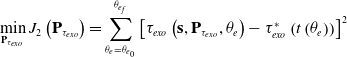 \begin{equation}\min _{\textbf{P}_{{\tau _{{exo}}}}} J_{2}\left(\textbf{P}_{{\tau _{exo}}}\right)=\sum _{\theta _{e}=\theta _{{e_{0}}}}^{\theta _{{e_{f}}}}\left[{\tau _{exo}}\left({\textbf{s},\textbf{P}_{{\tau _{exo}}}},{\theta _{e}}\right)-\tau _{exo}^{*}\left(t\left(\theta _{e}\right)\right)\right]^{2}\end{equation}
 \begin{equation}s.t.\colon \tau _{exo}\left(\textbf{P}_{{\tau _{exo}}},\theta _{e}\right)-\tau _{exo}^{*}\left(t\left(\theta _{e}\right)\right)=0, \theta _{e}=\theta _{{e_{0}}},\theta _{{e_{f}}}\end{equation}
This problem is solved using an SQP method in SNOPT [Reference Shepherd and Rouse23]. The second optimization is able to find the optimal torque control points for the exoskeleton torque $\tau _{exo}(\theta _{e})$
in terms of the encoder angle for lifting tasks.
$\tau _{exo}(\theta _{e})$
in terms of the encoder angle for lifting tasks.
In phase 2, based on the knee encoder angle during lifting, the optimal assistive torque is calculated from the B-spline interpolation function in real time using Eq. (24) in joint angle domain. This gives human knee joint an assistive torque. It is noted that the encoder angle must be within the given initial and final boundary conditions to provide optimal assistance. If it is outside the knee joint boundaries, a randomly selected small and safe constant assistive torque $\tau _{exo}=2.1$
Nm is provided.
$\tau _{exo}=2.1$
Nm is provided.
A comparison between exoskeleton torque obtained from B-spline interpolation ( $\tau _{exo}^{*}$
) and optimal exoskeleton torque profiles (
$\tau _{exo}^{*}$
) and optimal exoskeleton torque profiles ( $\tau _{exo}$
) are illustrated in Fig. 4. Figure 5 presents the optimal real-time exoskeleton torques with respect to knee joint angles with the maximum assistive torque as 6 Nm and 16 Nm, respectively.
$\tau _{exo}$
) are illustrated in Fig. 4. Figure 5 presents the optimal real-time exoskeleton torques with respect to knee joint angles with the maximum assistive torque as 6 Nm and 16 Nm, respectively.
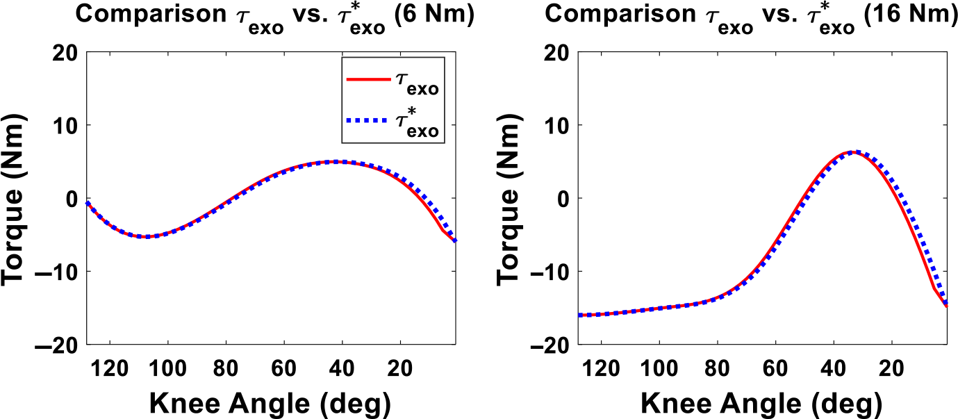
Figure 4. Comparison between B-spline interpolation and optimal exoskeleton torques as a function of human knee angles.
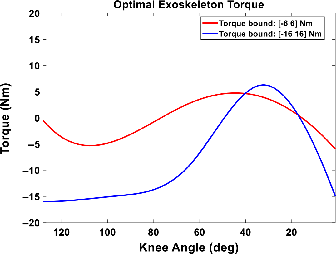
Figure 5. The optimal exoskeleton torque as a function of human knee angles during lifting. The knee joint angle starts from a squat position.

Figure 6. Lifting experiment setup without the exoskeleton.
4.2. Experimental procedure
The Institutional Review Board (IRB) approved the optimal control of the powered knee exoskeleton lifting experiment was conducted at Biodynamics Optimization and Motion Control Lab at Oklahoma State University. The test subject was a healthy 22-year-old male with no previous injuries, and a written consent form from the subject was taken before the experiment. The subject’s height and weight were 1.90 m and 81.36 Kg, respectively.
For this study, the subject had two lab visits. For the first visit, the subject’s anthropometric measurements were taken. Xsens motion capture system was used to obtain 3D kinematic data at 60 Hz, and the whole body sensors protocol was considered, as shown in Fig. 6. The Xsens system was first calibrated. Delsys Trigno EMG sensors were attached to the subject’s left leg and spine. For this experiment, the EMG activities of vastus medialis, vastus lateralis, and biceps femoris from the left leg and latissimus dorsi from the upper body were measured at 2000 Hz. The subject’s maximum voluntary contractions (MVCs) for the four muscles were measured for muscle activation normalization. In this study, three trials were conducted for each muscle at every MVC testing position [Reference Hamzaid, Smith and Davis42, Reference Wagner, Forister and Huot43]. A 30-s rest period was observed between two trials. The participant was instructed to exert his maximum force during each MVC testing session. For lifting task, the subject was instructed to lift an 11-Kg box without the exoskeleton with two feet standing on two Bertec force plates (Bertec, Columbus, Ohio, USA). However, the participant was allowed to choose his own lifting strategy. The lifting motion was recorded in Xsens’s MVN Analyze Pro software (MVN Awinda, Xsens Technologies BV, Enschede, the Netherlands). The GRFs were recorded using OptiTrack Motive 3.0 software (Natural Point, Corvallis, OR, USA) at 1000 Hz. In addition, EMGworks Acquisition (Delsys Inc., Natick, MA, USA) was used to collect and record the raw data of the EMG. The lifting task was repeated three times with a 3-min break between them. Next, the processed data from the MVN Analyze and Motive 3.0 were used to validate the simulation results against the experimental results without the exoskeleton. The recorded EMG data series were transferred to EMGworks Analysis (Delsys Inc., Natick, MA, USA) to obtain EMG activity in millivolts. Then EMG data series were further processed in MATLAB (MathWorks Inc., Natick, MA, USA), where data were bandpass-filtered with the cutoffs at 10–450 Hz, rectified, and then lowpass-filtered with a cutoff frequency of 6 Hz. Finally, the filtered EMG data series were normalized by the corresponding MVC EMG values. For processed GRFs, the average of two force plates was taken at each trial. Finally, we compared the average of the three experimental trials against the predicted data.
For the second visit, a light-weight, highly-back-drivable wearable knee exoskeleton developed by Picasso Intelligence, LLC, was used in this study. The unilateral mass of the exoskeleton was 2.25 Kg, and it could provide the maximum 25 Nm output torque. The exoskeleton’s smart motor included a motor, gear, driver, encoder, and controller. It used CAN bus protocol and was controlled by a teensy-based PCB board with a CAN bus chip. The proposed control strategy from Section 4.1 was implemented, and the code was uploaded to the teensy board of the exoskeleton control board. Finally, the subject was asked to wear Xsens whole body sensors, EMG sensors, and the exoskeleton to perform the lifting task again, as shown in Fig. 7. Similar to the first visit, the lifting motion was recorded in Xsens’s MVN Analyze Pro software, EMG raw data series were recorded in EMGworks Acquisition, and GRFs were recorded using OptiTrack Motive 3.0 software. A bluetooth-connected customized MATLAB GUI interface was used to collect the exoskeleton knee joint angle and knee joint torque. The lifting task was repeated three times, each with a 3-min break between them. The EMG data series were processed in EMGworks Analysis and MATLAB. Next, the processed data from the MVN Analyze, Motive 3.0, and Matlab GUI were used to validate the simulation results against the experimental results with the exoskeleton.
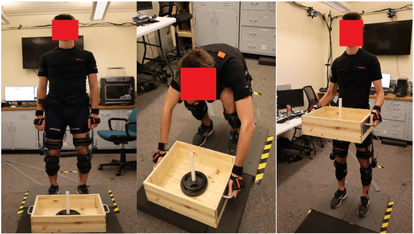
Figure 7. Lifting experiment setup with the exoskeleton.
5. Results
The lifting NLP problem is solved using an SQP method in SNOPT [Reference Gill, Murray and Saunders29]. The initial guess for the optimization is $\textbf{x}=\left[\begin{array}{c@{\quad}c} \textbf{P}_{\textit{human}}^{\mathrm{T}} & \textbf{P}_{\textit{current}}^{\mathrm{T}} \end{array}\right]^{\mathrm{T}}=[\textbf{0}]$
. For cubic B-spline interpolation, we use five control points (nctrl=5) for each joint. There are a total of 50 (n*nctrl) design variables and 217 nonlinear constraints for the lifting optimization without exoskeleton. The optimal solution is obtained in 0.59 s CPU time. The electrical and mechanical parameters of the DC motor are presented in Table II. For the lifting optimization with the exoskeleton, there are a total of 55 (n*nctrl+number of exo joints*nctrl) design variables and 222 nonlinear constraints. Two exoskeleton torque limits are considered in the optimization: [-6, 6] Nm and [-16, 16] Nm. The optimal solution is obtained in 1.51 and 1.54 s CPU time, respectively. An Intel® Core™ i7 2.11 GHz CPU and 16 GB RAM computer is used for the optimization. The input data for the box lifting task are given in Table III.
$\textbf{x}=\left[\begin{array}{c@{\quad}c} \textbf{P}_{\textit{human}}^{\mathrm{T}} & \textbf{P}_{\textit{current}}^{\mathrm{T}} \end{array}\right]^{\mathrm{T}}=[\textbf{0}]$
. For cubic B-spline interpolation, we use five control points (nctrl=5) for each joint. There are a total of 50 (n*nctrl) design variables and 217 nonlinear constraints for the lifting optimization without exoskeleton. The optimal solution is obtained in 0.59 s CPU time. The electrical and mechanical parameters of the DC motor are presented in Table II. For the lifting optimization with the exoskeleton, there are a total of 55 (n*nctrl+number of exo joints*nctrl) design variables and 222 nonlinear constraints. Two exoskeleton torque limits are considered in the optimization: [-6, 6] Nm and [-16, 16] Nm. The optimal solution is obtained in 1.51 and 1.54 s CPU time, respectively. An Intel® Core™ i7 2.11 GHz CPU and 16 GB RAM computer is used for the optimization. The input data for the box lifting task are given in Table III.
Table II. DC motor electromechanical parameters.
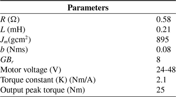
Table III. Task parameters for the lifting.

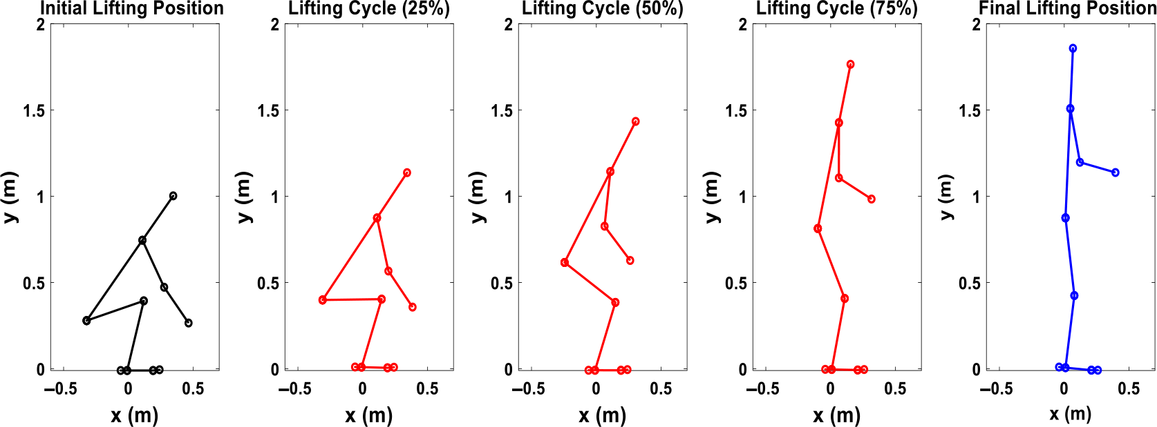
Figure 8. Simulation snapshots for 2D human 11 Kg box lifting without the exoskeleton.
5.1. Lifting validation without the exoskeleton
First, Fig. 8 illustrates the snapshots of the predicted lifting motion at different lifting times. Figure 9 compares experimental and simulation joint angles for the human spine, shoulder, elbow, hip, knee, and ankle joints. The horizontal and vertical GRFs are compared between experiments and simulation in Fig. 10.
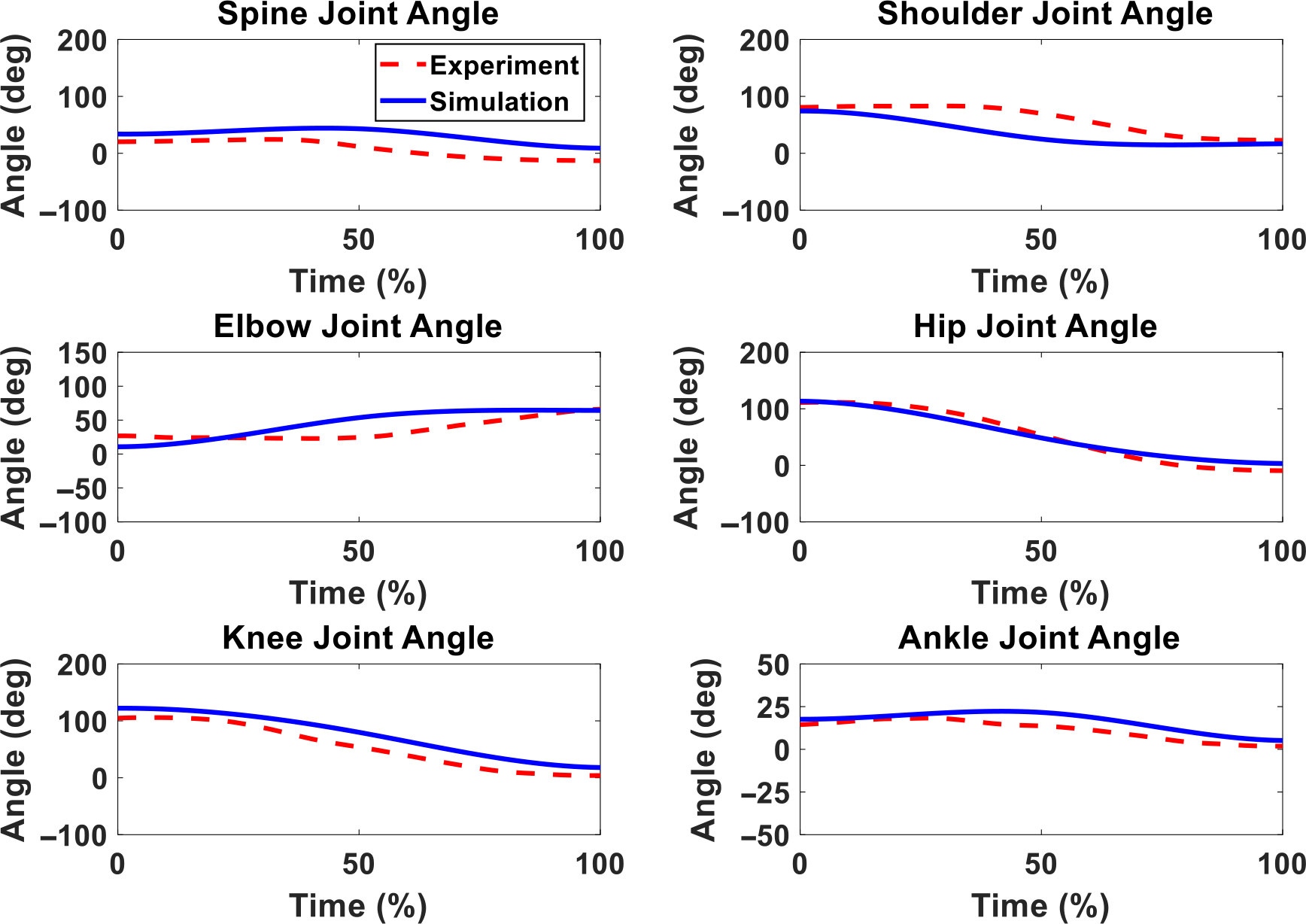
Figure 9. Human joint angle profiles comparison between simulation and experiment without exoskeleton for 11 Kg box lifting.

Figure 10. GRFs comparison of experiment and simulation without exoskeleton for 11 Kg box lifting.
5.2. Lifting validation with the exoskeleton
Figure 11 demonstrates the snapshots of the predicted lifting motion with 6 Nm maximum assistive torque. The optimization formulation predicts a similar lifting motion for the 16 Nm exoskeleton case as the motion of 6 Nm case in Fig. 11. The comparison of experimental and simulation joint angles for the human spine, shoulder, elbow, hip, knee, and ankle joints are presented in Figs. 12 and 13. Figures 14 and 15 compare the horizontal and vertical GRFs between experiments and simulations.

Figure 11. Simulation snapshots for 2D human lifting with optimal exoskeleton assistance, and the maximum assistive torque is 6 Nm.
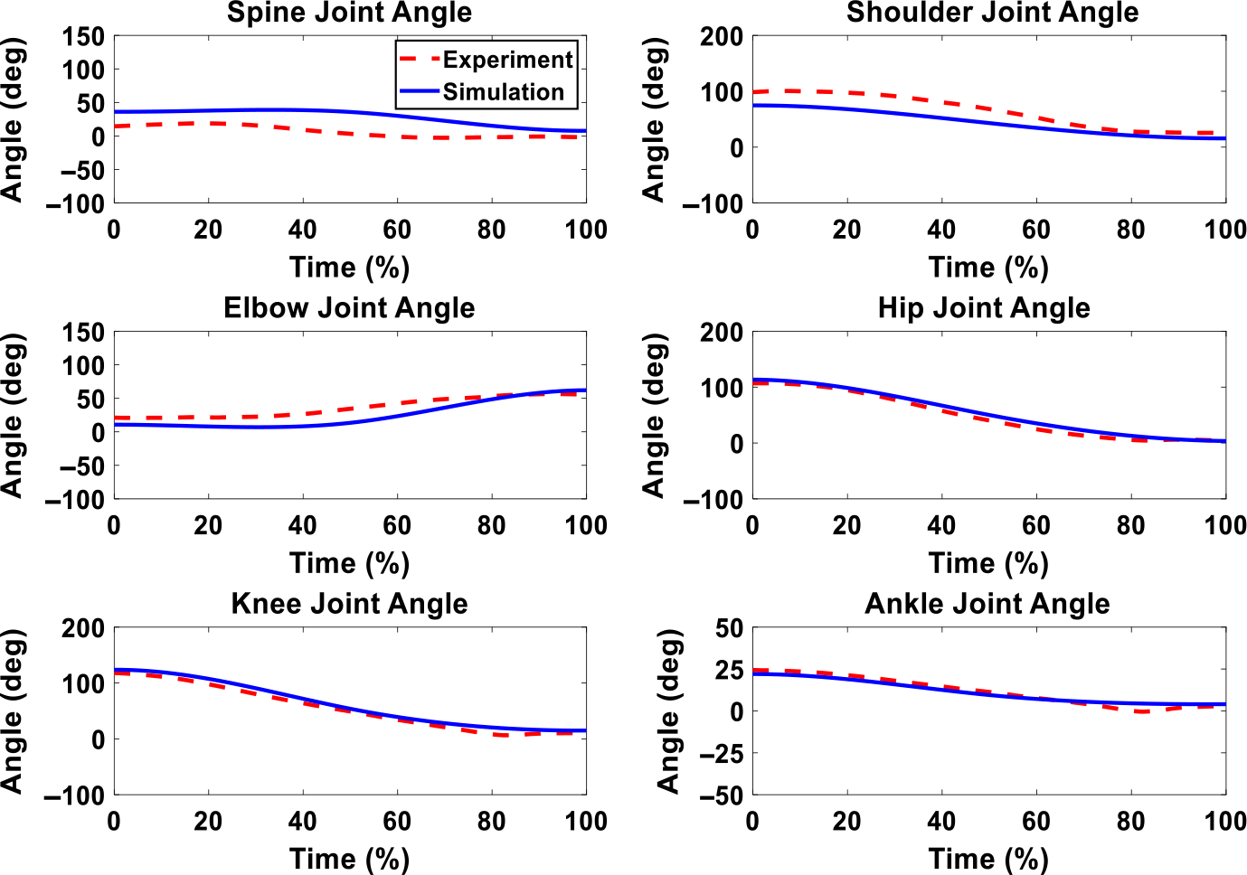
Figure 12. Human joint angles comparison between simulation and experiment with optimal exoskeleton torque, and the maximum assistive torque is 6 Nm.
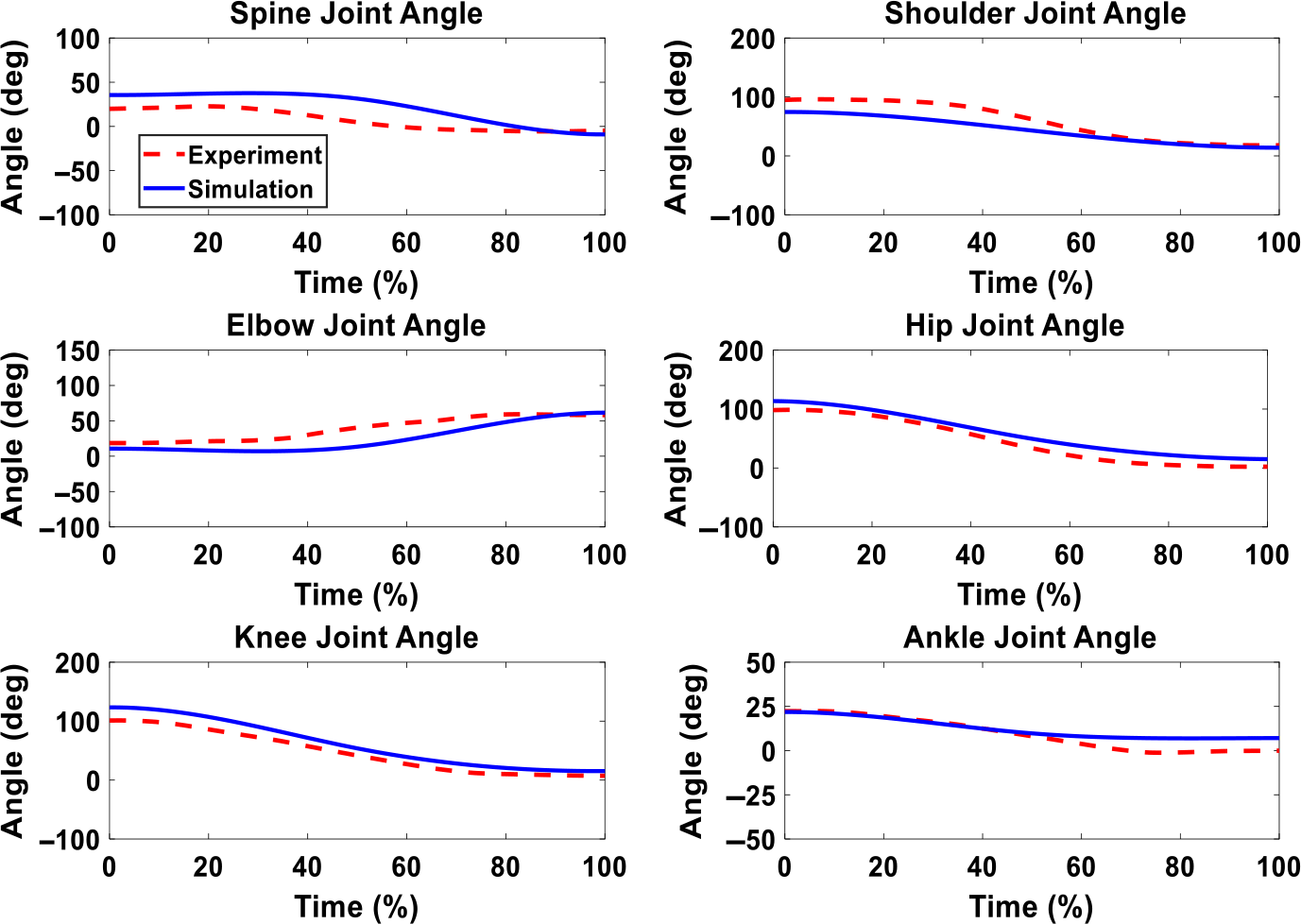
Figure 13. Human joint angles comparison between simulation and experiment with optimal exoskeleton torque, and the maximum assistive torque is 16 Nm.
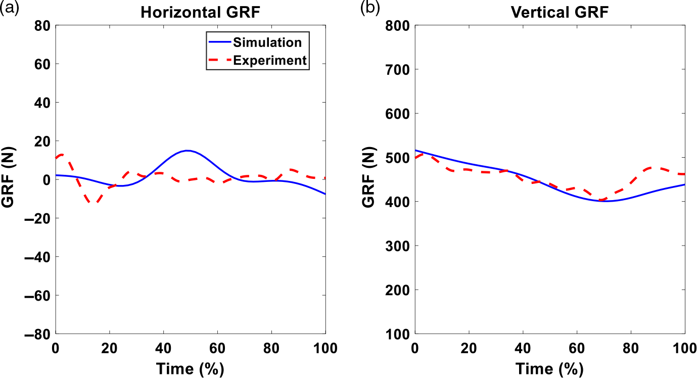
Figure 14. GRFs comparison of experiment and simulation with optimal exoskeleton torque, and the maximum assistive torque is 6 Nm.
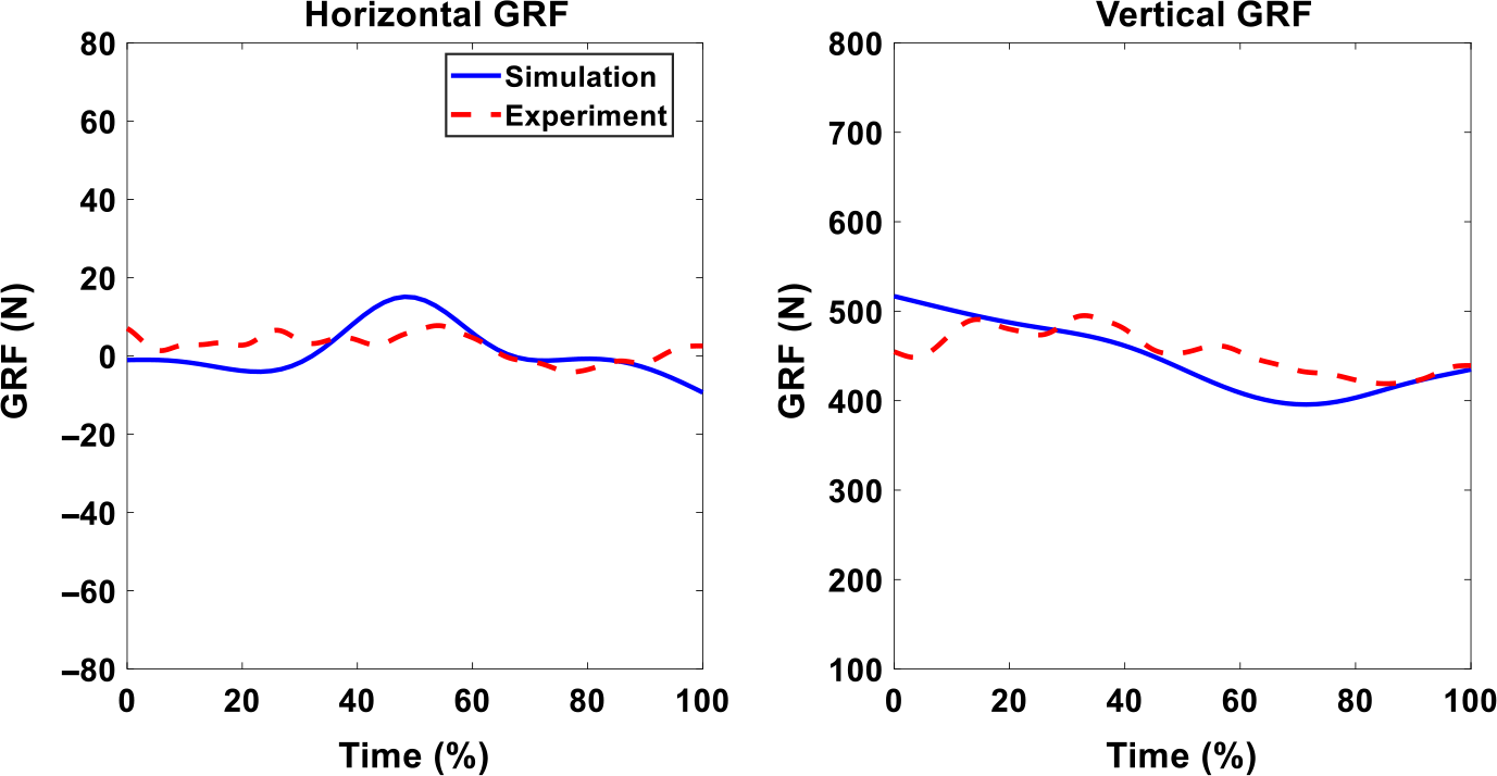
Figure 15. GRFs comparison of experiment and simulation with optimal exoskeleton torque, and the maximum assistive torque is 16 Nm.
5.3. Comparison of different assistive torque cases
We compare three cases in this section: without exoskeleton, exoskeleton with the 6 Nm maximum assistive torque, and exoskeleton with 16 Nm maximum assistive torque. The comparison of optimal human joint torques for the three cases is shown in Fig. 16. Figure 17 provides the comparison of experimental human joint angles. The GRFs of three cases are compared in Fig. 18. Finally, the comparisons of muscle activations are presented in Fig. 19.

Figure 16. Human joint torque simulation comparison of different cases (without an exoskeleton, maximum 6 Nm, and 16 Nm exoskeleton optimal assistances) for 11 Kg box lifting.
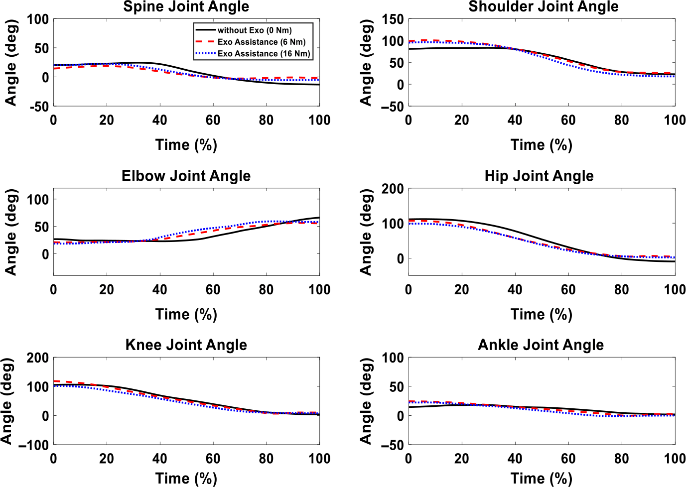
Figure 17. Human joint angles experimental comparison of different cases (without an exoskeleton, maximum 6 Nm, and 16 Nm exoskeleton optimal assistances) for 11 Kg box lifting.
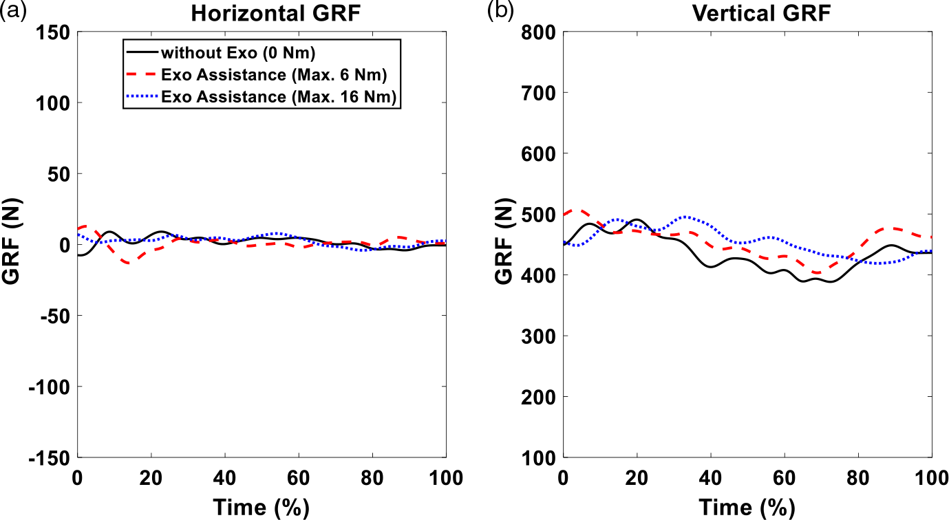
Figure 18. GRFs comparison of different cases (without an exoskeleton, maximum 6 Nm, and 16 Nm exoskeleton optimal assistances) for 11 Kg box lifting.
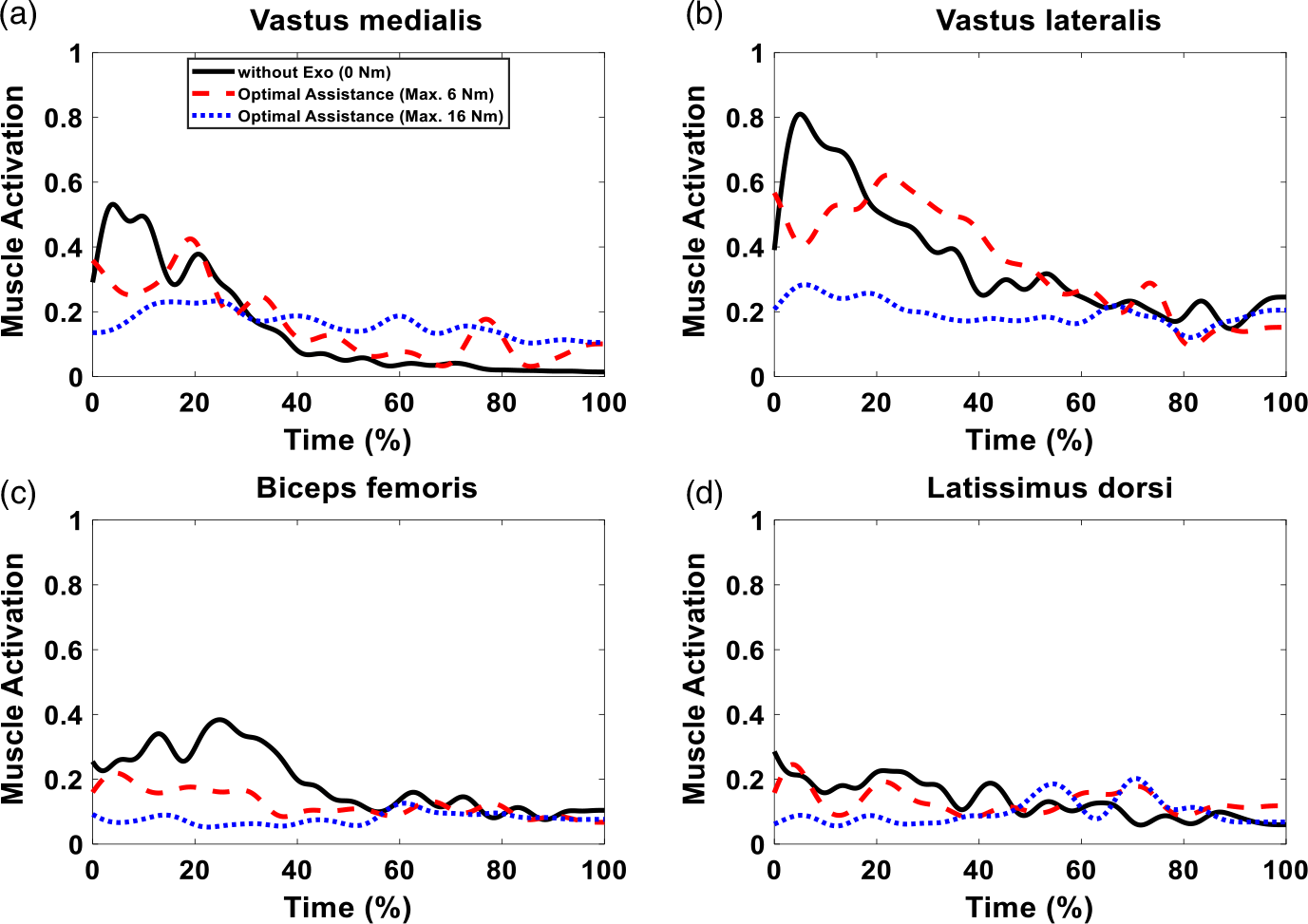
Figure 19. Muscle activations comparison of different cases (without an exoskeleton, maximum 6 Nm, and 16 Nm exoskeleton optimal assistances) for 11 Kg box lifting.
6. Discussion and conclusions
In this work, the snapshots of predicted lifting motion illustrate that the proposed lifting optimization formulation successfully predicts a natural lifting motion without exoskeleton as shown in Fig. 8. The predicted spine, hip, knee, and ankle joint angles are compared well with the experimental data in Fig. 9. However, there are some deviations for the spine, elbow, and shoulder joint angle profiles, and this may be due to less constraints imposed on the skeletal model’s upper body compared to the lower body. For example, the leg joint angle profiles have good predictions because the feet are fixed on the ground during lifting due to foot contact constraint. The predicted GRFs are reasonable, as shown in Fig. 10. The trends of simulation result closely follow the trends of the experiment data. However, the predicted vertical GRF values are higher than the experimental GRF until 80% of the lifting cycle but are within 2.27% of the experimental GRF.
For the lifting with exoskeletons, the optimization predicts the natural symmetric lifting motions for both optimal assistance cases, the maximum 6 Nm case (Fig. 11). We can observe the differences in lifting motion trajectories at 50% lifting cycle snapshots between liftings with and without exoskeletons (Fig. 8). With exoskeletons, the knee and elbow bend less at 50% lifting cycle compared to the case without exoskeleton. This clearly indicates that the lifting strategies have changed due to assistive torque. For joint angle comparisons (Figs. 12 and 13), for both cases, the predicted joint angle profiles show similar trends and magnitudes as the experimental data. We also notice larger discrepancies for upper body joints than the lower body joints. In addition, the predicted vertical GRFs are within 1.63% and 1.76% of the experimental GRFs, respectively, as shown in Figs. 14 and 15.
We can see the differences in joint torques between the cases without exoskeletons and the cases with exoskeletons, as shown in Fig. 16. However, for the cases with exoskeletons, only human knee joint torques have different values because different knee assistive torques are applied to knee joints. For other joints, the human torques are very similar because no exoskeletons are applied to those joints. It is observed that the actual peak human knee joint torque magnitudes decreased by 30.53% and 45.45% due to the exoskeleton assistance. In addition, the normalized cost function values (torque square) are 0.519, 0.438, and 0.413 for 0 Nm, the maximum 6 Nm, and the maximum 16 Nm optimal assistance cases. The human dynamic effort (cost function) is decreased by 15.61% and 20.42% with assistances compared to the lifting motion without exoskeleton. Therefore, knee assistive torque changes overall lifting motion trajectory and dynamic effort.
In Fig. 17, the joint angles have similar magnitudes and patterns for the cases with and without exoskeletons. In Fig. 18, horizontal GRFs have similar trends and magnitude for the cases with and without exoskeletons. For the vertical GRFs, without and with exoskeleton cases have similar trends during the lifting. For the maximum 16 Nm assistance case, the vertical GRF is higher than that of 0 Nm assistance case between 20% and 80% of the lifting cycle. For the maximum assistance of 6 Nm case, the vertical GRF is higher than that of 0 Nm assistance case during the entire lifting process. The exoskeleton motor is attached to thigh and shank through wrapped frames. Therefore, the forces generated by the exoskeleton motor are applied to the human thigh and shank to assist lifting. This causes variations in the vertical GRFs for knee exoskeletons.
We consider three muscles (knee extensor: vastus medialis and vastus lateralis; knee flexor: biceps femoris) from the lower extremity and one spine muscle (latissimus dorsi) from the upper extremity for muscle activation comparison, as shown in Fig. 19. The trends of the muscle activations are similar for the cases with and without exoskeletons for the lifting task. However, the exoskeletons significantly reduce these muscle activations for the maximum 16 Nm assistive torque case. It is observed that the peak values of vastus medialis, vastus lateralis, biceps femoris, and latissimus dorsi are reduced by 56.05%, 64.98%, 67.15%, and 29.13%, respectively. For the maximum 6 Nm assistive torque case, only biceps femoris’ activity is reduced significantly, and the peak value is reduced by 42.82%. Furthermore, the mean values of muscle activations for vastus medialis, vastus lateralis, biceps femoris, and latissimus dorsi are 0.161, 0.346, 0.123, and 0.132, respectively, for the 6 Nm case. These mean values are changed to 0.163, 0.197, 0.079, and 0.099 for the 16 Nm case. Correspondingly, for the case without exoskeleton, the mean values of muscle activations are 0.149, 0.356, 0.192, and 0.134, respectively. It is observed that for vastus lateralis, biceps femoris, and latissimus dorsi muscles, the exoskeleton decreases the activations by 3.00%, 35.61%, and 2.06%, respectively, for the 6 Nm case, and 44.65%, 58.98%, and 26.39%, respectively, for the 16 Nm case. It is worth noting that although the peak value of vastus medialis muscle activation decreases by the exoskeletons, the mean value increases by small amounts of 8.11% and 9.69% for the 6 and 16 Nm cases, respectively.
In this study, we used an inverse dynamics optimization to predict the human-exoskeleton symmetric lifting motion, then the optimal exoskeleton torque was transferred in joint angle domain to control the powered exoskeleton in real time. The optimal control of knee exoskeleton was implemented to provide optimal assistance to the human knee joint for lifting. The overall method worked well, and the simulation results were reasonably matched with the experimental data. In summary, the proposed optimal control method is subject-specific and has the capability to reduce human torques and muscle activations. As a result, dynamic human effort and injuries can be mitigated by using the proposed optimal control of the powered knee exoskeleton during object lifting. The limitations of this work are that we only consider the squat lifting strategy and a single subject for the experiment. For future work, we will also investigate the stoop lifting technique. In addition, we will validate the control strategy and lifting optimization by collecting more data from subjects with different percentiles and gender. We also plan to develop the learning-based approach by training an artificial neural network (ANN) based on the simulation results to provide real-time optimal assistance for lifting tasks.
Acknowledgments
The authors would like to thank the participant for the experimental data collection for this work.
Author contributions
A.A. and Y.X. contributed to the study conception and design. A.A. performed data collection and analysis. A.A. and Y.X. wrote the main manuscript text. Y.X. supervised this work. All authors read and approved the final manuscript.
Financial support
This study is supported by Research Jumpstart/Accelerator Grant from Oklahoma State University.
Competing interests
The authors declare none.
Code or data availability
No.
Ethical standards
The authors assert that all procedures contributing to this work comply with the ethical standards of the relevant national and institutional committees on human experimentation and with the Helsinki Declaration of 1975, as revised in 2008.


 Open access