


INTRODUCTION
The Quaternary covers the past 2580 ka. Human evolution largely occurred during this period, which is characterized by a dynamic climate, dominated by alternating glacial and interglacial conditions driven by orbital forcing. The Quaternary climate is often studied to contextualize Earth's ongoing and future climate changes, and their effects on the cryosphere and sea level fluctuations—topics of crucial scientific, societal, and political relevance.
Most paleo-climatology, -geomorphology, and -glaciology studies have focused on the most recent portion of the Quaternary (i.e., the last glacial-interglacial cycle). Those that have ventured beyond the last cycle have been particularly interested in the coldest and warmest “extremes” of the many glacial-interglacial cycles that characterized the Quaternary (e.g., looking for an analogue of the current interglacial). This was especially true some thirty years ago, when, in order to counter this excessive focus on Quaternary “extremes,” a popular paper (Porter, Reference Porter1989, cited >200 times) advocated the need to shift attention to “average” Quaternary conditions, which were calculated using the then available oxygen isotope record. It was suggested that, while most climate and, especially, glacial research had only described culminations of glacial and interglacial phases (the “extremes” noted above), conditions were actually intermediate between these states for most of the Quaternary. It was also argued that these “average” conditions affected landscape evolution far more than the extremes, and glacial landscapes around the world therefore reflect evolution under “average” conditions. Through the use of three isotope records from marine sediment cores, it was calculated that the “average” Quaternary glacial conditions were last met ca. 12,000 yr BP (i.e., during the Younger Dryas stadial), and were generally associated with an equilibrium-line altitude (ELA) depression of ~500 m, roughly half-way between the last glacial maximum (LGM) ELA and the present-day ELA. The glacial cirques of the US Cascade Range (which have a Younger Dryas ELA ~450 m above the LGM and ~450 m below the modern), as well as the fjords of Norway, were presented amongst the most spectacular examples of the influence of “average” Quaternary glacial conditions on landscape evolution.
The concept of “average” Quaternary conditions continued to gain popularity in subsequent decades, particularly in relation to the glacial buzzsaw hypothesis. This suggests that mountain height is controlled by the long-term average ELA, which represents an upper limit on the growth of topography, breached only by a small number of “lightning rod” peaks (Brozović et al., Reference Brozović, Burbank and Meigs1997). Studies have used the correlation between peak altitudes and “average” Quaternary ELA (often coinciding with cirque floor elevations) to support the glacial buzzsaw hypothesis (e.g., Mitchell and Montgomery, Reference Mitchell and Montgomery2006; Foster et al., Reference Foster, Brocklehurst and Gawthorpe2008; Mitchell and Humphries, Reference Mitchell and Humphries2015).
Now, thirty years since Porter (Reference Porter1989) first introduced the concept, and with much improved Quaternary climate (and ice volume) proxy data (Lisiecki and Raymo, Reference Lisiecki and Raymo2005), it is perhaps time to revisit the idea of an “average” Quaternary condition.
METHODS
The marine δ18O record represents the ratio between the stable 18O and 16O isotopes. This record, when measured on benthic foraminifera fossils extracted from deep-sea sediment cores, is arguably the most complete and commonly used proxy for climate and glacial conditions during the Quaternary, because it quantifies changes in global ice volume and deep water temperatures, which are controlled by high-latitude atmospheric temperatures. In simple terms, the cooler the climate, the more 16O becomes trapped in glacial ice. With the preferential removal of 16O, the oceans become enriched in 18O, which is recorded in the carbonate tests constructed by benthic foraminifera. Hence, under colder conditions with larger global ice volumes, δ18O in benthic foraminifera will be elevated (relative to a standard), while the opposite happens during warmer/reduced ice volume conditions. In this paper, we use the LR04 δ18O stack, generated from 57 globally distributed benthic δ18O records (Lisiecki and Raymo, Reference Lisiecki and Raymo2005; Fig. 1), which is considered the most comprehensive δ18O dataset available to date. The data are provided in the form of a benthic δ18O value (per mil, or ‰), at 1000-year time steps. For the sake of clarity, and to avoid any potential misunderstanding, we will refer to “mean” values in our calculations, instead of “average,” because the former has a clear statistical, arithmetic meaning, whereas “average” is often used when referring to something “usual” or “typical.”
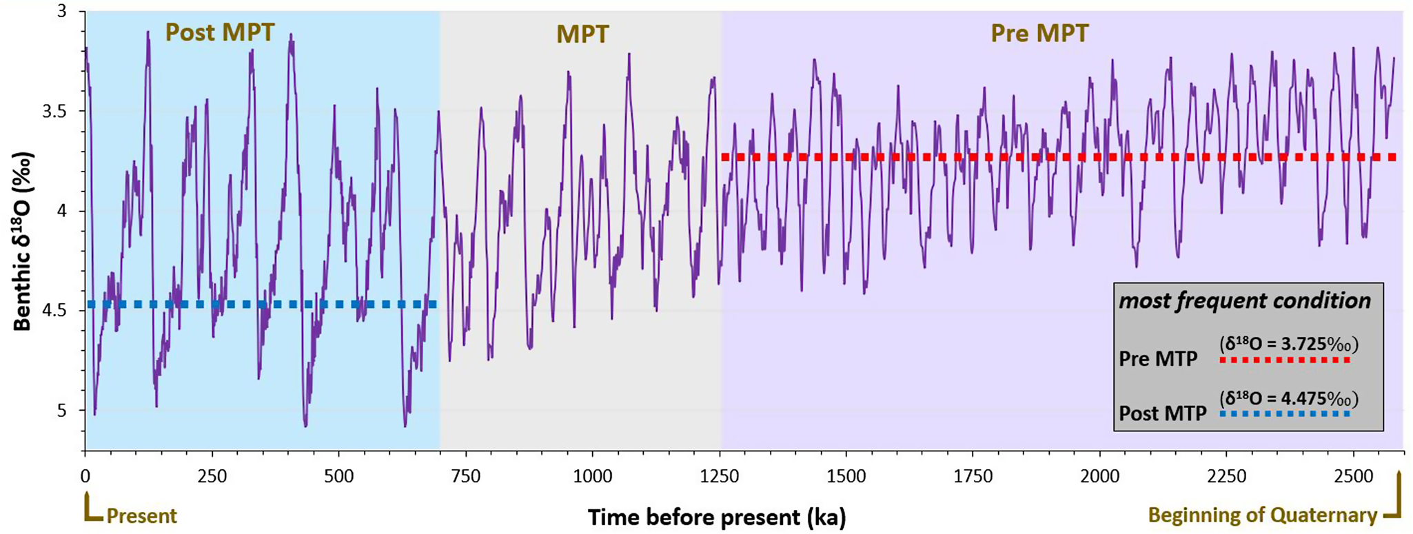
Figure 1. The Quaternary δ18O curve obtained from 57, globally distributed, benthic δ18O records (derived from data in Lisiecki and Raymo, Reference Lisiecki and Raymo2005). The curve has been split into its three most distinct climatic periods: before, during, and after the Middle Pleistocene Transition (pre-MPT, MPT, and post-MPT). The dashed blue line shows the most-frequent δ18O post-MPT, while the dashed red line refers to the most-frequent δ18O pre-MPT.
RESULTS
The Quaternary is characterized by many climate oscillations, generally alternating between glacial and interglacial conditions, in a seemingly regular fashion. However, the δ18O curve (Fig. 1) shows that the amplitude and frequency of these climatic oscillations have changed through time (Shackleton and Opdyke, Reference Shackleton, Opdyke, Cune and Hays1976). Specifically, prior to 1250 ka, the amplitude of climate oscillations was relatively smaller, and their frequency higher, following an obliquity-dominated ca. 41 ka cycle. Over the past 700 ka, the amplitude of the climatic oscillations has been much higher, and their frequency has decreased to the eccentricity-forced ca. 100 ka cycle, with an increasingly pronounced asymmetry between the long slow build up to the glacial maxima and the rapid deglaciation into the interglacials. Between 1250 and 700 ka, the amplitude and frequency of oscillations changed considerably (Clark et al., Reference Clark, Archer, Pollard, Blum, Rial, Brovkin, Mix, Pisias and Roy2006). This transitional phase is referred to as the Middle Pleistocene Transition (MPT, 1250–700 ka), while the most recent time will be referred to here as post-MPT, and the earlier phase as pre-MPT.
Given the above tripartite division of the δ18O curve (Fig. 1), it is immediately apparent that a single mean value for the Quaternary (δ18O = 3.97‰) is not a particularly informative parameter to characterize the climatic and glacial conditions of the past 2580 ka. Instead, at least two separate mean values should be considered, one pre-MPT (2580–1250 ka, mean δ18O = 3.73‰) and one post-MPT (700–0 ka, mean δ18O = 4.16‰), while it may be argued that the transient nature of the MPT itself makes the extraction of a mean δ18O value for this period essentially meaningless (Table 1).
Table 1. Summary statistics of key parameters from the Quaternary δ18O curve, as discussed in the paper. Note that the most-frequent values are calculated using bin sizes of 0.05‰.
Mean or most-frequent conditions?
The relative regularity of the pre- and post-MPT climatic oscillations suggests that the mean δ18O values have some relevance. However, given the continuous oscillatory nature of climate throughout the Quaternary and the presence of various, small anomalies even in the amplitude and frequency of the relatively regular pre- and post-MPT δ18O glacial-interglacial cycles, there is no guarantee that these mean values represent the most typical, or frequent, climatic and glacial conditions. This is important in relation to the potential influence that these mean conditions could have had on long-term landscape evolution. It is therefore apparent that an alternative (perhaps better) approach would be to take into consideration the most-frequent, rather than the mean, condition.
A relatively simple calculation allows us to identify the most-frequent δ18O of 3.725 ± 0.025‰ for the pre-MPT period, and 4.475 ± 0.025‰ for the post-MPT (frequencies are calculated with δ18O bin sizes of 0.05‰; Fig. 2), with the latter, in particular, differing considerably from the corresponding post-MPT mean value (Table 1).
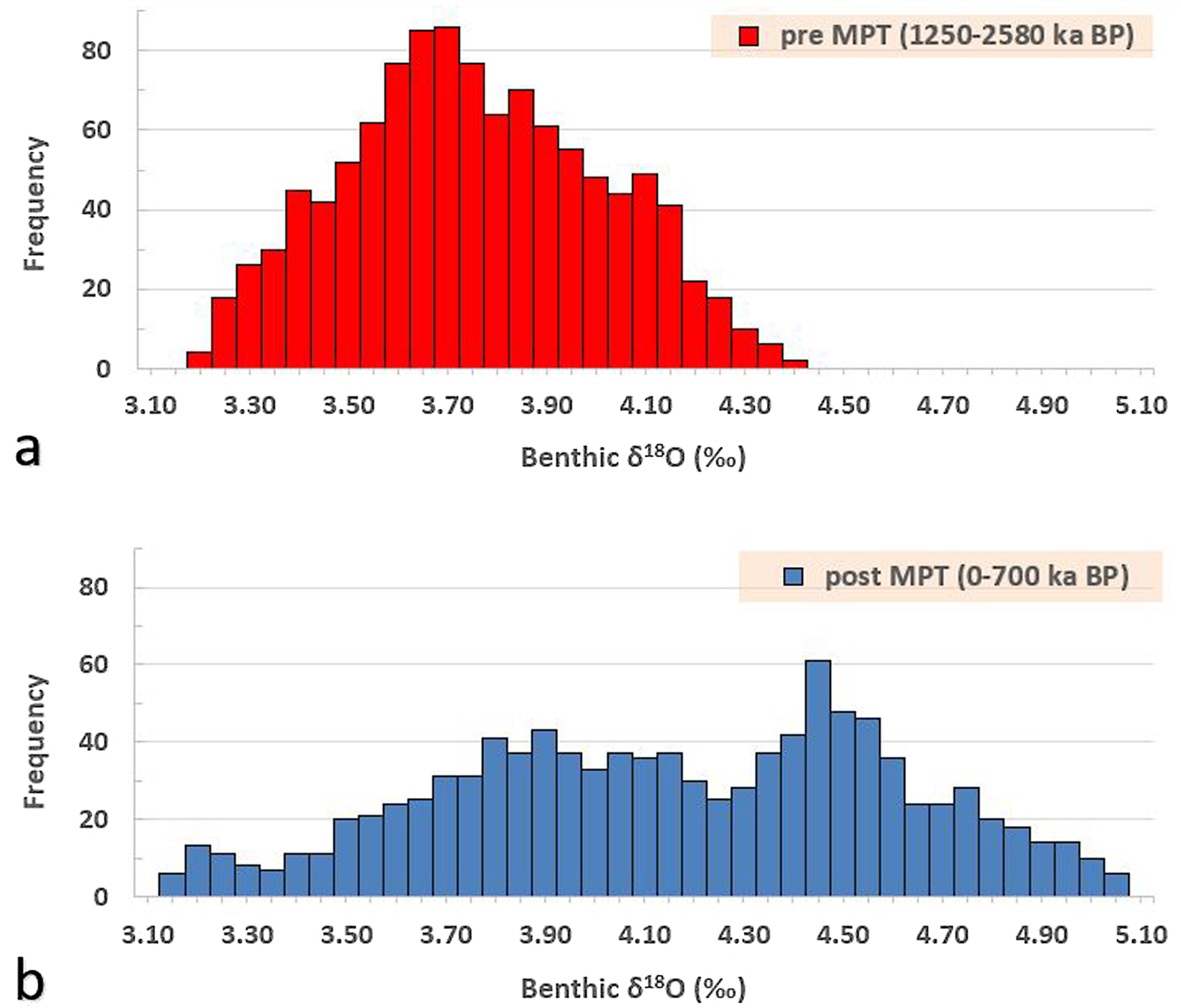
Figure 2. The frequency distribution of δ18O values (a) pre- and (b) post-MPT.
How frequent were these most-frequent conditions?
The pre-MPT frequency peak of δ18O = 3.725 ± 0.025‰ occurred 86 times throughout the pre-MPT Quaternary, while the mean occurrence is 43.8 times, and 30% of all pre-MPT δ18O values occurred at least 64 times (Fig. 2; Table 1). The post-MPT frequency peak of δ18O = 4.475 ± 0.025‰ occurred 61 times throughout the post-MPT Quaternary, while the mean occurrence is 26.4 times, and 30% of all post-MPT δ18O values occurred at least 36 times (Fig. 2; Table 1). It is not possible to easily translate these frequencies into exact lengths of time, because the data have a temporal resolution of 1 ka. Moreover, within any given cycle, δ18O tends to rise more steeply than it descends. However, it is assumed, as a first approximation, that each occurrence of a δ18O value lasted no more than 1 ka, given the temporal interval of the original data. Therefore, the most-frequent pre-MPT climate condition lasted no more than 86 ka, or 6.4% of the entire pre-MPT period. Similarly, the most-frequent post-MPT condition lasted no more than 61 ka, or 8.7% of the post-MPT period.
When did these conditions last occur?
The climatic conditions represented by the pre-MPT frequency peak, δ18O = 3.725 ± 0.025‰, and the post-MPT frequency peak, δ18O = 4.475 ± 0.025‰, last occurred during 11.31–11.47 ka (i.e., during the warming period that characterized the Younger Dryas stadial to Holocene transition) and 14.81–15.04 ka (i.e., end of the Oldest Dryas stadial), respectively (Table 1). These age values are determined from the δ18O curve, assuming a linear relationship between successive δ18O values at 1 ka time steps.
DISCUSSION
Progressing on from the concept of a mean Quaternary condition
Porter (Reference Porter1989) correctly pointed out that too much attention had been given to the “extreme” conditions (e.g., glacial maxima and interglacial warmest periods) of Quaternary climate. However, the oscillatory, but not perfectly regular and transient, nature of climatic and glacial conditions that characterized the past 2580 ka suggests that the concept of mean condition is equally misleading. Specifically, there have been at least three distinct climate periods through the Quaternary. The MPT was transitional, so a mean value here is worthless. The pre-MPT had relatively consistent amplitude and frequency of oscillations, although δ18O (slightly) increased throughout the period, which also partly undermines a focus on mean conditions. The post-MPT is arguably the most regular (stable) of all three periods, with relatively consistent frequency and amplitude of δ18O oscillations, and consideration of its mean conditions may therefore be of relevance. However, there are still a number of minor fluctuations within each glacial/interglacial cycle. A focus on the most-frequent (longest lasting) conditions, therefore, seems to be a better approach, especially if the purpose is to establish the climatic and glacial scenario that had the strongest influence on long-term landscape evolution.
Putting the most-frequent condition and its potential geomorphological expression into perspective
It is challenging to determine with certainty if pre- and/or post-MPT most-frequent conditions left a trace on our present-day landscape, although the relatively recent evolution of geochronological and modeling techniques applied to the study of long-term landscape evolution has been very helpful with unraveling this puzzle (e.g., Strunk et al., Reference Strunk, Knudsen, Egholm, Jansen, Levy, Jacobsen and Larsen2017). In general, the relative influence of pre- and post-MPT conditions on the present-day landscape might depend on whether a specific landform or landscape is mostly erosional or depositional, and on its chances of preservation at these temporal scales, largely dictated by its morphoclimatic setting. The issue of preservation is, of course, particularly acute for “pre-MPT landscapes,” given that they underwent 1250 ka of MPT and post-MPT climatic oscillations characterized by a different amplitude, frequency, and most-frequent δ18O than they experienced during pre-MPT times, which could have modified the pre-MPT landscape entirely.
However, it is possible, at least in theory, that some landscapes might have evolved quickly at the beginning of the Quaternary and changed little thereafter. For example, this has been advocated for glacial cirques (e.g., Fig. 3), where morphology may have been shaped mostly by initial and final glacial conditions of each early Quaternary glacial cycle, rather than by the (mean or) most-frequent condition (Barr et al., Reference Barr, Ely, Spagnolo, Evans and Tomkins2019). Other landscapes (or landforms) may have experienced the opposite (i.e., evolving slowly at the beginning of the Quaternary), possibly because the landscapes were mantled by a protective regolith layer that had to be removed before bedrock erosion could proceed (Clark and Pollard, Reference Clark and Pollard1998). However, many (most?) landscapes are likely to have evolved continuously through time and what we see today represents the cumulative effect of the many glacial and interglacial cycles of the past 2580 ka, not to mention the many landscape features that were inherited from timescales of considerably longer duration than the Quaternary. This final scenario of an ever-evolving Quaternary landscape is best seen in environments dominated by depositional processes, but modeling outputs suggest that pre-MPT landscape evolution can also affect post-MPT glacial erosion (Pedersen and Egholm, Reference Pedersen and Egholm2013).
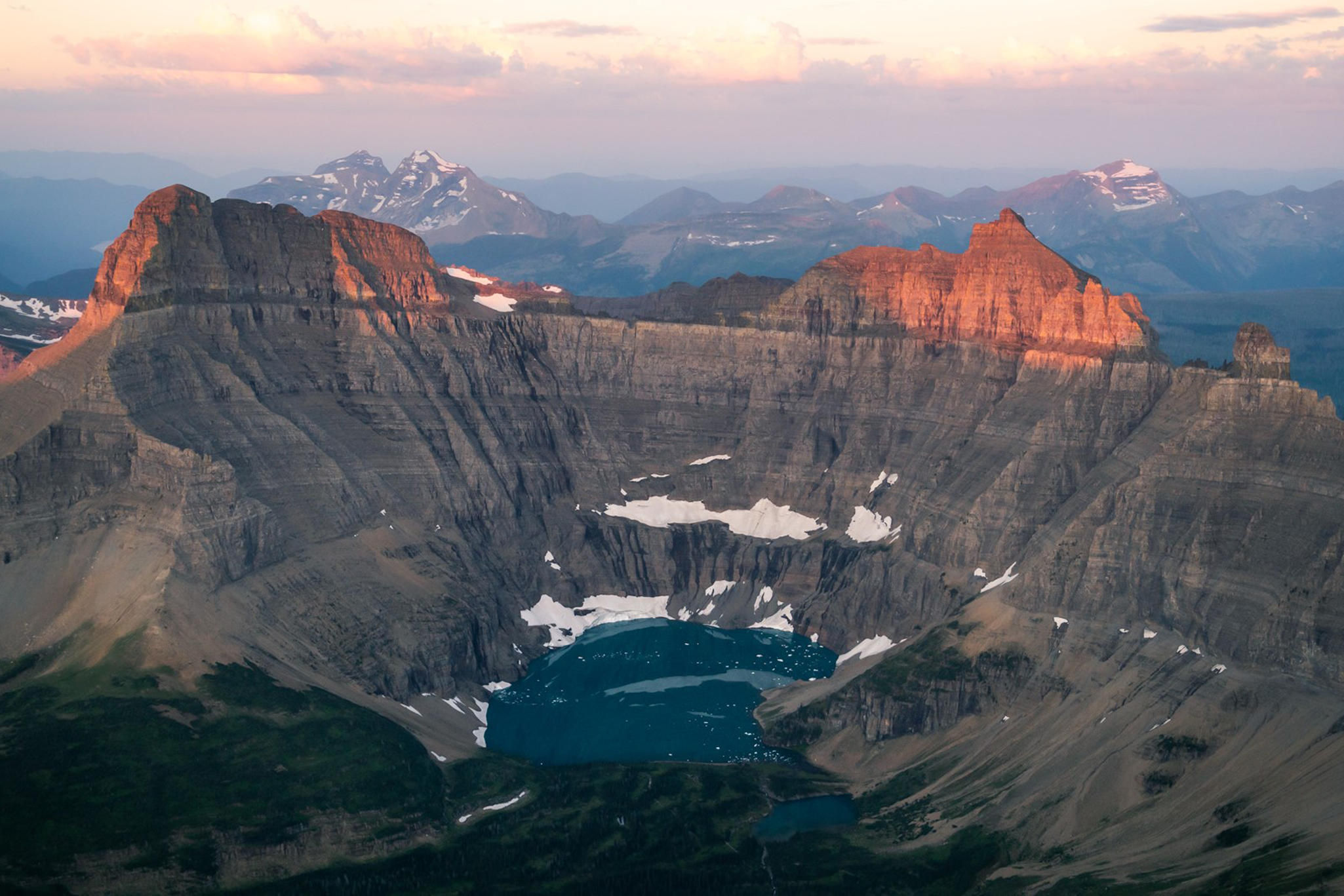
Figure 3. A spectacular example of glacial erosion: the cirque of Iceberg Lake, Montana, USA. Photo courtesy of Scott Krunz (www.scott-kranz.com, August 2016).
Although all of the above remain realistic scenarios, the potential importance of the most-frequent pre- or post-MPT climatic/glacial conditions on present-day landscape can be discussed further based on our results. These indicate that: (1) most-frequent pre- and post-MPT conditions happened about twice as often as the mean occurrence of all other δ18O values; (2) many other δ18O values occurred a similar number of times to the most-frequent condition; and (3) each frequency peak occurred for only <9% of the entire pre- or post-MPT duration. Thus, it seems rather unlikely that these most-frequent climate conditions have imparted a noticeable geomorphological expression in the present-day landscape. Indeed, our analysis indicates that the most-frequent post-MPT condition last occurred at the end of the Oldest Dryas stadial, while the most-frequent pre-MPT condition last occurred at the Younger Dryas stadial to Holocene transition. Neither of these times stand out particularly as being associated with landforms or landscapes that could be attributed to the cumulative effect of erosional or depositional processes.
A further consideration is that the temporal response of geomorphological processes to the same climate forcing, inferred from the δ18O record, might have differed regionally. This is certainly the case for glacial conditions and associated processes, which had a profound influence on many present-day landscapes. The δ18O curve is particularly dependent on the cyclical growth of the Laurentide ice sheet, but it is not so well synchronized with the behavior of other ice masses of different sizes and dynamics (Gibbard and Hughes, Reference Gibbard and Hughes2020). This is demonstrated, for example, by the timing of the last glacial maxima, which differed across the planet (Hughes et al., Reference Hughes, Gibbard and Ehlers2013). Thus, the most-frequent conditions extracted from the δ18O curve might have had an expression in the North American landscape, but not necessarily so in other regions worldwide.
Topography, and elevation in particular, would also play a considerable modulating role in determining dominant processes, and their morphological expression, for any given global climate condition, even within a single region. Rather than focusing on “unique” mean or most-frequent conditions, an alternative approach to the study of the connection between Quaternary climate and today's landscapes would be to consider how long, within the past 2580 ka, a specific landscape was under the dominating influence of a specific climate-driven process. For example, in relation to glacial processes, how long a sector of a mountain chain was covered by ice, ideally with a distinction between erosive (warm) and non-erosive (cold) basal ice conditions, versus how long it was exposed subaerially to paraglacial processes.
Finally, while the δ18O record is arguably our best continuous (throughout the Quaternary) proxy for global ice volume and atmospheric temperature, it is important to stress that the landscape is influenced by climatic factors more widely, for example by parameters such as precipitation, seasonality, etc., that are not fully incorporated into the δ18O record.
Problems with the use of a Quaternary “average” ELA in buzzsaw hypothesis testing
The concept of an “average” Quaternary condition has been extended to the definition of an “average” Quaternary ELA, which has been used to test the glacial buzzsaw hypothesis (which suggests that glacial erosion limits the elevation/growth of mountains). The ELA represents the elevation at which the amount of mass gained by a glacier, usually via snowfall, equals the amount of ice lost, generally by ablation, in a yearly budget. ELA can be measured on modern glaciers or calculated from the reconstruction of former glaciers. Despite its simple definition, ELA represents a powerful, quantitative expression of the relationship between glaciers and climate. Since a glacier's ELA is determined by contemporary climate, a paleoglacier's ELA can be used to assess paleoclimate (e.g., Rea et al., Reference Rea, Pellitero, Spagnolo, Hughes, Ivy-Ochs, Renssen, Ribolini, Bakke, Lukas and Braithwaite2020). With glacial erosion often assumed to be highest at, or just below, a mountain glacier's ELA (but see Brocklehurst and Whipple, Reference Brocklehurst and Whipple2006), the idea that an “average” Quaternary ELA could be used to test the glacial buzzsaw hypothesis has attracted attention in recent decades (e.g., Mitchell and Montgomery, Reference Mitchell and Montgomery2006; Foster et al., Reference Foster, Brocklehurst and Gawthorpe2008; Anders et al., Reference Anders, Mitchell and Tomkin2010; Mitchell and Humphries, Reference Mitchell and Humphries2015). Given the link between ELA and climate, it would be possible, locally, to define a mean/most-frequent ELA based on the Quaternary δ18O curve (e.g., by calculating the ELA during the period most recently characterized by the mean or most-frequent Quaternary δ18O value). This is essentially what a number of studies (e.g., Mitchell and Humphries, Reference Mitchell and Humphries2015) have done when, following Porter (Reference Porter1989), they defined a local “average” Quaternary ELA as the midpoint between the LGM stadial ELA and modern ELA, which in some places roughly corresponds to the ELA during the Younger Dryas stadial. A correlation of “average” ELA, elevation of maximum erosion (identified through hypsometric studies), and peak elevation has then been used as evidence of the glacial buzzsaw (e.g., Foster et al., Reference Foster, Brocklehurst and Gawthorpe2008).
Our results suggest that such approaches are problematic for a number of reasons. First, rather than focusing on an average ELA, it would be better to consider the most-frequent ELA. In principle, this could be estimated using the ELA from a paleoglacier reconstruction relating to the most recent occurrence of the most-frequent Quaternary condition, the latter obtained from the δ18O curve (in the absence of a better, local climate/glacial proxy). Second, this approach should not be applied to regions that underwent significant elevation change during the Quaternary (e.g., due to isostasy or tectonics). Third, rather than using a single value for the Quaternary, the focus should be on the pre- and post-MPT most-frequent ELAs. Given that neither the most-frequent pre- nor post-MPT conditions last occurred during the Younger Dryas stadial, calculation of the “average” ELA should not rely on finding the mid-point between the LGM stadial and modern ELAs. Fourth, the significance of the most-frequent ELA is limited by the fact that many other ELAs occurred a similar number of times, so that (pre-/post-MPT) glacial erosion was most likely maximized within a relatively large interval of ELAs, rather than a single value.
CONCLUSION
Porter's (Reference Porter1989) intuition that Quaternary climate extremes have had little influence on present day landscape is likely correct, and particularly relevant since many landscape reconstructions tend to focus on these extremes, indirectly suggesting that what happened in-between is of secondary importance. However, our study indicates that a focus shift to “average” Quaternary conditions is equally questionable. In particular, our analysis, based on the most comprehensive LR04 δ18O stack (Lisiecki and Raymo, Reference Lisiecki and Raymo2005), indicates the following. (1) Because the frequency and amplitude of climate oscillations are not constant throughout the Quaternary, separate mean δ18O values should be considered for the pre- and post-MPT periods, within which glacials and interglacials alternated in a seemingly regular fashion. (2) Mean values are not necessarily indicative of the most-frequent conditions, the latter being most relevant in terms of potential influence on the evolution of the landscape. Hence, a better approach is to extract, and focus on, the most-frequent (and cumulatively longest-lasting) δ18O values for the pre- and post-MPT time intervals. (3) Because of the oscillatory nature of the Quaternary climate, the most-frequent pre- and post-MPT conditions lasted for <9% of the entire pre- and post-MPT time spans, and many other δ18O values occurred at similar frequencies. (4) In many locations, it is likely that present-day landscape reflects, at least in part, processes that occurred during the Quaternary. In some cases, the landscape could have evolved quickly, before the MPT, and then slowed down after the MPT; in other cases, the opposite may have occurred; and in most instances the landscape has been evolving continually prior to and through the Quaternary. However, given point (3) above, it is unlikely that the (mean and) most-frequent conditions had a major effect on long-term landscape evolution and left a widespread, significant geomorphological signature on the present-day topography. (5) By extension, an excessive focus on an “average” Quaternary ELA, a parameter often used to test the glacial buzzsaw hypothesis, is also problematic and certainly the idea that “glacial conditions broadly intermediate between those of today and those of the last glacial maximum dominated the Quaternary Period” (Porter, Reference Porter1989, p. 251) is not substantiated by our study. (6) Overall, with regards to their potential influence on the landscape and use in landscape evolution models, it may be better to consider using a range of most-frequent conditions for each of the pre- and post-MPT periods, rather than a “unique” mean or most-frequent value, for example by looking at the 30% most-frequent pre-MPT conditions (corresponding to a δ18O interval of 3.55–3.90). (7) Finally, consideration should be given to the fact that the temporal geomorphological response to the same inferred climate forcing might have differed regionally. For example, regional records might be more informative than global ones when it comes to establishing the most-frequent glacial condition, and its landscape expression.
Acknowledgments
We would like to acknowledge the constructive feedback received by Lewis Owen, Jamie Shulmeister, Phil Gibbard, and an anonymous reviewer. We are also grateful to photographer Scott Krunz (www.scott-kranz.com) for his permission to use the beautiful image of Figure 3.


 Open access