


1 Introduction
In the study of collisionless plasmas, when dealing with scales comparable to ion characteristic time and length scales, it is essential to take into account ion kinetic effects. Of course, a fully kinetic approach that utilizes solutions of the Vlasov equation for both the ion and the electron component of the plasma provides a fundamental description. However, it is often the case that the plasma consists of suprathermal ions and thermal electrons, e.g. due to selective ion energization, or the electron scales are irrelevant, for example in the propagation of slow ion-acoustic waves. In such cases, a viable alternative is to use a hybrid model that treats only the ion component kinetically. A particularly successful model which has been utilized in order to study various processes that involve ion scales, is the hybrid Vlasov–Maxwell model with kinetic ions and massless fluid electrons (Valentini et al. Reference Valentini, Trávníček, Califano, Hellinger and Mangeney2007; Tronci Reference Tronci2010; Servidio et al. Reference Servidio, Valentini, Califano and Veltri2012; Cerri et al. Reference Cerri, Califano, Jenko, Told and Rincon2016; Franci et al. Reference Franci, Cerri, Califano, Landi, Papini, Verdini, Matteini, Jenko and Hellinger2017). As this model has been used in several kinetic simulations to study physical processes, such as magnetic reconnection, kinetic turbulence and shearing flows, the problem of constructing consistent equilibrium states that can serve as reliable initial conditions in stability and dynamics calculations, arises. It is common practice in the literature to use Maxwellian and shifted Maxwellian distribution functions as initial conditions. However, in collisionless plasmas, it is anticipated that the distribution functions of the kinetic species deviate from the Maxwellian distribution. Using incorrect or off-equilibrium initial conditions in numerical simulations, stability analysis and wave propagation studies, can lead to unphysical behaviour. In particular, when studying wave propagation it is crucial to use exact equilibria to avoid spurious oscillations that can arise from the use of shifted Maxwellian distribution functions (Malara, Pezzi & Valentini Reference Malara, Pezzi and Valentini2018).
Numerous spacecraft measurements and observations have revealed that large amplitude, localized electrostatic structures known as Bernstein–Greene–Kruskal (BGK) modes are prevalent in space plasmas, where they manifest as solitary wave structures in both the magnetosphere and the solar wind (Matsumoto et al. Reference Matsumoto, Kojima, Miyatake, Omura, Okada, Nagano and Tsutsui1994; Ergun et al. Reference Ergun, Carlson, McFadden, Mozer, Muschietti, Roth and Strangeway1998). Theoretically, BGK modes arise as solutions to the Vlasov–Poisson system and were first proposed by Bernstein, Greene and Kruskal (Bernstein, Greene & Kruskal Reference Bernstein, Greene and Kruskal1957). Their existence has been verified through numerical simulations (Demeio & Holloway Reference Demeio and Holloway1991) and experimental observations (Fox et al. Reference Fox, Porkolab, Egedal, Katz and Le2008). Although they are usually interpreted as electron phase space holes (Hutchinson Reference Hutchinson2017), recent observations from NASA's Magnetospheric Multiscale (MMS) Mission (Burch et al. Reference Burch, Moore, Torbert and Giles2016) have revealed the presence of a new type of bipolar electrostatic structures observed in a supercritical quasiperpendicular Earth's bow shock crossing by the MMS. These structures have been interpreted as ion BGK modes or ion phase space holes (Vasko et al. Reference Vasko, Mozer, Krasnoselskikh, Artemyev, Agapitov, Bale, Avanov, Ergun, Giles and Lindqvist2018, Reference Vasko, Wang, Mozer, Bale and Artemyev2020; Wang et al. Reference Wang, Vasko, Mozer, Bale, Artemyev, Bonnell, Ergun, Giles, Lindqvist and Russell2020), as they are produced by monopolar negative electrostatic potentials and their formation is attributed to the ion two-stream instability arising from the interaction of incoming and reflected ions. In light of these observations, a theory of ion phase-space holes was recently proposed in Aravindakshan et al. (Reference Aravindakshan, Yoon, Kakad and Kakad2020), which builds upon earlier studies by Schamel (Reference Schamel1971), Schamel (Reference Schamel1986), Ng & Bhattacharjee (Reference Ng and Bhattacharjee2005) and Chen, Thouless & Tang (Reference Chen, Thouless and Tang2004). Within this framework the electrons are considered adiabatic and the dynamics of their distribution function is neglected. This is due to the fact that the velocities of ion BGK modes are significantly slower than the electron thermal velocity. However, like the standard theory of BGK modes, this approach is purely electrostatic and does not take into account the magnetic field or the interaction with a background plasma component. In the last two decades, there have been significant developments in the theory of BGK modes incorporating magnetic fields (Ng, Bhattacharjee & Skiff Reference Ng, Bhattacharjee and Skiff2006; Allanson, Wilson & Neukirch Reference Allanson, Wilson and Neukirch2016b; Ng Reference Ng2020), since the magnetic field plays an important role in the environments where BGK modes are observed.
In this work, we adopt the abovementioned hybrid fluid-kinetic model to construct equilibria that take into account the self-consistent effects of magnetic fields and can be interpreted as quasineutral BGK modes. When dealing with wave structures characterized by large time and length scales, i.e. ones much larger than the electron time and the Debye length scale, there is sufficient time for the electrons to rearrange accordingly so that the hybrid approach and the quasineutrality condition are physically plausible. By employing this model we implicitly assume that the length scale of the wave is comparable to the ion inertial length $\ell _i$ , i.e. much larger than the Debye length $\ell _D$
 . Thus, the model is not well-suited for describing smaller bipolar structures such as the ion holes observed by the MMS mission during Earth's bow shock crossing, as these structures have spatial scales up to 10 $\ell _D$
 (Vasko et al. Reference Vasko, Wang, Mozer, Bale and Artemyev2020). In future work, we will investigate possible improvements to our model, that would allow for the construction of electrostatic structures with length scales $\sim \ell _D$
 and nonzero charge separation. For now, our focus is mainly on the impact of magnetic field variations and contributions stemming from fluid electrons on the formation of ion kinetic waves. Thus, we consider waves with characteristic lengths of approximately $\ell _i$
 and neglect the self-consistent charge separation. A similar approach was employed in Tasso (Reference Tasso1969) to study the problem of electrostatic BGK modes, demonstrating that the quasineutrality condition ensures the positivity of the trapped particle distribution function. To construct stationary states, we assume planar spatial symmetry and consider distribution functions that depend on the particle constants of motion, ensuring that the Vlasov equation is satisfied. Then we solve an inhomogeneous Beltrami equation that arises from the generalized Ohm's law of the model, upon assuming that the electrons are described by Boltzmann distributions. This is essentially an integro-differential equation that can be turned into a differential equation for the vector potential components if the form of the distribution function is specified, or conversely, into an integral equation for the distribution function upon defining the magnetic field. Within this framework, the electrostatic potential can be determined by the quasineutrality condition as a function of the vector potential components (e.g. see Mynick, Sharp & Kaufman Reference Mynick, Sharp and Kaufman1979; Tasso & Throumoulopoulos Reference Tasso and Throumoulopoulos2014; Kuiroukidis, Throumoulopoulos & Tasso Reference Kuiroukidis, Throumoulopoulos and Tasso2015).
The electron contribution, given by $\lambda \boldsymbol {B}$ in Ampere's law (an inhomogeneous Beltrami equation), has some interesting ramifications. One such example is the modulation of the shape and distribution of the bipolar electric field pulses, which can be linked to spatial fluctuations of the magnetic field, caused by the electron current. A nonzero Beltrami parameter can lead to the emergence of multiple localized ion phase-space holes, even when the free parameters and initial conditions are set up to avoid such structures for $\lambda = 0$
 . In addition, we have noticed that these structures exhibit periodicity for ion distribution functions that are symmetric in the two particle momentum constants of motion associated with the two ignorable coordinates. However, under suitable selection of initial conditions and for asymmetric distribution functions they appear in an irregular and chaotic manner. Both observations can be explained by examining the Hamiltonian phase-space structure of the dynamical system that governs the spatial evolution of the magnetic field and vector potential components. This system originates from the generalized Beltrami–Ampere equation and the definition of the vector potential. More specifically, we show that these equations form a noncanonical Hamiltonian system (see e.g. Morrison Reference Morrison1998) that can be canonized under an appropriate transformation. The two-degree of freedom system possesses a first integral of motion, namely the Hamiltonian function. However, for symmetric ion distribution functions, there exists an additional integral, similar to the angular momentum, and the system is thus integrable. For asymmetric distribution functions though, this additional integral does not exist, and the orbits in parts of the phase-space become non-integrable and chaotic. This is not surprising as it is well-established that magnetic field lines form Hamiltonian systems (Morrison Reference Morrison2000) of more than one degree-of-freedom, which are typically chaotic. Furthermore, chaotic behaviour is not unexpected in the context of kinetic equilibria. Previous studies, such as Ghosh et al. (Reference Ghosh, Janaki, Dasgupta and Bandyopadhyay2014), have reported similar behaviour of magnetic fields in Vlasov–Maxwell equilibria. However, our analysis is more general than that of Ghosh et al. (Reference Ghosh, Janaki, Dasgupta and Bandyopadhyay2014) because we prove the Hamiltonian nature of the equilibrium system for a wider class of distribution functions. Also, our analysis is concerned with the hybrid Vlasov–Maxwell model that treats the electrons as a massless fluid. In terms of equilibria, this translates into an electron current density of the form $\lambda \boldsymbol {B}$
 . The electron contribution gives rise to Coriolis-like (gyroscopic) coupling terms in the Hamiltonian system, which alter significantly the dynamics of the system as illustrated by various Poincaré surfaces of section. An interesting modification induced by the electron current is that unbounded trajectories of the Hamiltonian system can be confined by considering nonzero values of $\lambda$
 .
.
The rest of the paper is structured as follows. In § 2, we derive the quasineutral hybrid Vlasov model from a parent non-quasineutral model using appropriate ordering. Section 3 describes the general method for constructing equilibrium solutions, further specializing to the one-dimensional (1-D) case. In § 4, we demonstrate that the equations governing the equilibrium magnetic field form a noncanonical Hamiltonian system that can be transformed into a canonical one under an appropriate change of variables. In § 5, we select a particular distribution function and numerically integrate the magnetic field equilibrium equations and we use Poincaré surfaces of section to study the phase-space structure. In § 6, we provide a paradigm for constructing analytic equilibria by specifying the pseudopotential associated with the Hamiltonian system, rather than the distribution function. The distribution function is subsequently reconstructed using a Hermite polynomial expansion method. Finally, in § 7, we summarize the results and propose future extensions of the present study.
2 The hybrid model and equilibrium formulation
In the study of slow electrostatic structures like ion BGK modes, which propagate with the ion acoustic velocity, electron dynamics can be neglected and the electrons can be treated adiabatically. This is possible because the electron thermal velocities are typically much greater than the ion acoustic velocity, making electron particle–wave resonances and other kinetic effects irrelevant. To study such cases we can start our analysis with a hybrid Maxwell-Vlasov system that accounts for massless electrons and allows for charge separation,


where $f$ is the ion distribution function, $\sigma$
 is the charge density given by

the current density is

where the kinetic ion current is

and other symbols are standard. To close the system we assume an isothermal electron fluid, i.e. $T_e=T_{e0}={\rm const}$ . The Gauss law (2.5) can be used for determining the electron density $n_e$
 .
.
Stationary solutions of the system (2.1)–(2.6), can be found upon setting $\partial /\partial _t =0$ , while travelling wave structures can be studied by a Galilean transformation from the laboratory frame. Thus, we consider the following system of equilibrium equations:


The system (2.10)–(2.14) can describe a wide variety of physical processes ranging from ion BGK modes to nonlinear Alfvén waves. To see this let us consider two different normalization schemes. The first scheme involves a normalization in terms of microscopic characteristic quantities, such as the ion Debye length, introducing the following nondimensional quantities:

where $n_0$ is a characteristic background density, $T_{i0}$
 is a characteristic ion temperature and

are the ion Debye length and the ion thermal velocity, respectively. In terms of these nondimensional quantities, upon dropping the tildes, (2.10)–(2.14) become


where $\tau = T_{e0}/T_{i0}$ , $\beta _{th,i}^2=v_{th,i}^2/c^2$
 and $P_e=n_e$
 .
.
In the nonrelativistic limit where $\beta _{th,i}^2=v_{th,i}^2/c^2 \rightarrow 0$ the system (2.17)–(2.20) reduces to the Vlasov–Poisson system for the ions, while the electrons are adiabatic with their particle density described by the Boltzmann distribution

which has been used in previous studies for the description of ion holes (Aravindakshan et al. Reference Aravindakshan, Yoon, Kakad and Kakad2020) (note that upon taking the limit $\kappa \rightarrow \infty$ in Eq. (5) of Aravindakshan et al. (Reference Aravindakshan, Yoon, Kakad and Kakad2020), one recovers (2.21)). Therefore, with this particular ordering, magnetic field effects in the ion hole formation can be introduced upon keeping terms of the order $\beta _{th,i}^2$
 .
.
Now, let us consider an alternative normalization, which is more suitable in cases where the magnetic fields are strong and charge separation is insignificant,

where $B_0$ is a characteristic value of the magnetic field modulus and

are the ion inertial length, the Alfvén velocity and the ion cyclotron frequency, respectively.
With this normalization, the system (2.10)–(2.14) reads as follows:


In the above equations, $\kappa =k_B T_{e0}/(mv_A^2)$ and $\beta _A^2:= v_A^2/c^2$
 . By using this ordering scheme, in the nonrelativistic limit where $\beta _A^2 \rightarrow 0$
 , the Gauss law implies the quasineutrality condition $n_i=n_e$
 and we obtain a system of equilibrium equations for the ordinary quasineutral hybrid Vlasov–Maxwell system (e.g. see Malara et al. Reference Malara, Pezzi and Valentini2018). Here, when effects due to charge separation cannot be neglected, we need to keep terms of the order $\beta _A^2$
 .
.
3 Equilibrium solutions
In this section we consider the system (2.24)–(2.27) in the limit $\beta _A^2\rightarrow 0$ . Within this framework we will calculate certain quasineutral, 1-D equilibria where all equilibrium quantities depend on a single spatial coordinate, denoted by $x$
 . To study the equilibrium problem one can in general exploit the pressure tensor formulation (e.g. see Mynick et al. Reference Mynick, Sharp and Kaufman1979; Harrison & Neukirch Reference Harrison and Neukirch2009; Allanson et al. Reference Allanson, Neukirch, Troscheit and Wilson2016a). Specifically, we begin by considering the first velocity moment of the Vlasov equation (2.24), giving

where

is the ion pressure tensor. Upon inserting the generalized Ohm's law (2.25) into (3.1) and using the quasineutrality condition we find

This equation can be seen either as a differential equation for determining the magnetic field $\boldsymbol {B}$ upon specifying $f$
 , or as an integral equation to determine $f$
 upon specifying $\boldsymbol {B}$
 .
.
For the rest of the paper we will consider 1-D equilibria assuming that all physical quantities depend only on one cartesian coordinate $x$ , while the distribution function can depend on all three velocity coordinates $(v_x,v_y,v_z)$
 . This consideration is physically relevant as various measurements of space plasmas have revealed that certain wave structures, e.g. BGK modes in the Earth's bow-shock (e.g. Vasko et al. Reference Vasko, Mozer, Krasnoselskikh, Artemyev, Agapitov, Bale, Avanov, Ergun, Giles and Lindqvist2018; Wang et al. Reference Wang, Vasko, Mozer, Bale, Artemyev, Bonnell, Ergun, Giles, Lindqvist and Russell2020) are nearly 1-D structures, in the sense that the electric field is highly polarized. In this case the force-balance equation (3.3) yields

where $P_{xx}$ is the $xx$
 component of the ion pressure tensor and $n=n_i=n_e$
 :
:


Equation (3.4) is a pressure balance equation, where the first, second and third terms in the left-hand side of the first equality correspond to the ion, electron and magnetic pressure, respectively. Equation (3.4) can be seen also as an expression for the energy conservation of a pseudoparticle with velocity components $B_y=-\textrm {d}A_z/{\textrm {d} x}$ and $B_z=\textrm {d}A_y/{\textrm {d} x}$
 moving in a pseudopotential $V=P_{xx}+\kappa n$
 . Thus, the energy (Hamiltonian) of the pseudoparticle is ${\mathcal {H}} = B^2/2 + P_{xx}+\kappa n$
 .
.
An equilibrium state of a 1-D hybrid Vlasov system should satisfy (3.4). As the $y$ and $z$
 coordinates are ignorable, the corresponding canonical momenta,


are particle constants of motion of the kinetic ions, as is the energy $H=v^2/2+\varPhi$ . Note that the canonical momenta have been written in non-dimensional form, normalizing the vector potential as $\tilde {\boldsymbol {A}}=\boldsymbol {A}/(v_AB_0/\varOmega )$
 , and that $H$
 is different from ${\mathcal {H}}$
 . The former refers to the physical energy of the kinetic ions while the latter represents the energy of the pseudoparticle whose velocity corresponds to the equilibrium magnetic field. By Jean's theorem, any function of $p_y$
 , $p_z$
 and $H$
 will solve the Vlasov equation (3.15). This can be easily verified by substituting $f=f(H,p_y,p_z)$
 in the Vlasov equation expressed in Cartesian spatial and velocity coordinates.
The final step to fully define the equilibrium problem is to introduce a relation that connects the electron density with the electrostatic potential. This is usually done through the quasineutrality condition. Although we have used quasineutrality to replace the electron density $n_e$ with the ion density $n_i=n$
 , the equation $n_i=n_e$
 cannot be used to determine $\varPhi$
 in terms of $A_y$
 , $A_z$
 , since there is no information about how the number density of the electrons is related to $\varPhi$
 , $A_y$
 and $A_z$
 . To overcome this problem we can define quasineutrality in a way similar to Mynick et al. (Reference Mynick, Sharp and Kaufman1979), i.e.

We can show, however, (see Harrison & Neukirch Reference Harrison and Neukirch2009) that $\partial P_{xx}/\partial \varPhi = -n$ and therefore (3.9) reads

which is satisfied by number density functions of the form

where $W$ is an arbitrary function of $A_y$
 and $A_z$
 . If we require now the components $J_{ky}$
 and $J_{kz}$
 of the kinetic current density to be given by partial derivatives of the pseudopotential $V$
 with respect to $A_y$
 and $A_z$
 , respectively, we have


where we have used $\partial P_{xx}/\partial A_y = J_{ky}$ and $\partial P_{xx}/\partial A_z = J_{kz}$
 (Mynick et al. Reference Mynick, Sharp and Kaufman1979; Harrison & Neukirch Reference Harrison and Neukirch2009). Equations (3.12) and (3.13) imply $W(A_y,A_z) =\textrm {const.}$
 and therefore the number density is described by a Boltzmann distribution of the form

Note that in the calculations above we consider $\varPhi$ , $A_y$
 and $A_z$
 as being independent, although $\varPhi$
 can be expressed in terms of $A_y$
 and $A_z$
 through $\textrm {e}^{\varPhi /\kappa }W(A_y,A_z)=\int \,\textrm {d}^3v f(H,p_y,p_z)$
 , as will be the case in the next section.
With (3.14) we can readily see that the system (2.24)–(2.27) splits into


This splitting implies that the electron current density is $\lambda \boldsymbol {B}$ , i.e. it is aligned with the magnetic field. This is justified by the fact that inertialess electrons move along the magnetic field lines. Note that in general the coefficient $\lambda$
 , which will be called the Beltrami or Coriolis parameter, may be a function of some spatial coordinate. In this case though, the following equations should be satisfied by $\lambda$
 :
:

or

since $\boldsymbol {\nabla }\boldsymbol {\cdot } \boldsymbol {J}_k =0$ at equilibrium. In the 1-D case, (3.16) reduces to a system of two integro-differential equations for determining $A_y$
 and $A_z$
 , These equations are


where


and $\lambda$ is a constant parameter. If the distribution function is a function of the form $f=f(H,p_y,p_z)$
 , the Vlasov equation and consequently (3.4) are satisfied automatically.
4 Equilibrium equations as a Hamiltonian system
4.1 Hamiltonian structure
Since the 1-D equilibrium magnetic field can be represented by the velocity of a pseudoparticle with conserved energy, it is natural to seek for a Hamiltonian structure in the equilibrium equations. The second-order system composed of (3.19)–(3.20) can be reduced to a first-order system of ordinary differential equations using $\boldsymbol {B}=\boldsymbol {\nabla }\times \boldsymbol {A}$ , viz.


Let us consider distribution functions of the special form

where $g$ is an arbitrary but well-behaved and positive function of the two canonical momenta. With this choice, the particle and current densities are given by


where

Integration with respect to $H$ yields


At this point we use the quasineutrality condition $n_i=n_e$ rather than assuming $\varPhi =0$
 which was the case in other studies (e.g. Ghosh et al. Reference Ghosh, Janaki, Dasgupta and Bandyopadhyay2014; Allanson et al. Reference Allanson, Neukirch, Troscheit and Wilson2016a). Upon imposing quasineutrality and using (3.14) we have

Using (4.10) and solving for the electrostatic potential $\varPhi$ yields

where

Upon inserting the expression (4.14) for the electrostatic potential into (4.11)–(4.12), we can show that

that is, the two components of the current density can be derived from the function

as

This same result was obtained in Channell (Reference Channell1976) and Mynick et al. (Reference Mynick, Sharp and Kaufman1979) for $\varPhi =0$ and $\varPhi \neq 0$
 . Note that the pseudopotential $V$
 is in fact $V=(\kappa +1) \tilde {n} =(\kappa +1)\tilde {P}_{xx}$
 , where $\tilde {n}=n(\varPhi (A_y,A_z),A_y,A_z)$
 and $\tilde {P}_{xx}=P_{xx}(\varPhi (A_y,A_z),A_y,A_z)$
 . Hence, (3.4) yields

Now, for $V$ to be a valid potential function it should satisfy

which can easily be verified from (4.17). Therefore, it can be seen that the dynamical system (4.1)–(4.4) is a noncanonical Hamiltonian system, i.e. it is of the form

where $\boldsymbol {\xi } = (A_y,A_z,B_z,-B_y)$ , ${\mathcal {J}}$
 is a $4\times 4$
 noncanonical Poisson matrix of the form

where $0_2$ and $I_2$
 are the $2\times 2$
 zero and identity matrices, respectively, and the Hamiltonian function is given by (4.19). Note that in the Hamiltonian framework, the conservation of ${\mathcal {H}}$
 is a consequence of the antisymmetry of the Poisson matrix $\boldsymbol {{\mathcal {J}}}$
 . Also, the structure of the Poisson matrix implies that the Hamiltonian system can be canonized by the following change of variables $\boldsymbol {\xi }=(A_y,A_z,B_z,-B_y)\rightarrow \boldsymbol {\xi }_c=(Q_1,Q_2,P_1,P_2)$
 , where

When expressed in the variables $\boldsymbol {\xi }_c$ , the system (4.1)–(4.4) takes the form

where

and

We observe that for $\lambda \neq 0$ , the Hamiltonian of the canonical system possesses two Coriolis-like coupling terms that would be absent if the contribution of the electrons in the current density vanished. Those terms, would also be absent if we had considered the solely kinetic Vlasov–Maxwell system rather than the hybrid variant with fluid, massless electrons. Such Coriolis couplings arise in Hamiltonian models of finite Larmor radius stabilization (Morrison & Kotschenreuther Reference Morrison and Kotschenreuther1990), plasma streaming instabilities (Kueny & Morrison Reference Kueny and Morrison1995), fluid models that describe collisionless magnetic reconnection (Tassi et al. Reference Tassi, Morrison, Waelbroeck and Grasso2008) and galactic dynamics (Binney & Tremaine Reference Binney and Tremaine2008; Salas et al. Reference Salas, Lanchares, Iñarrea and Farrelly2022), and play a significant role in the dynamical evolution of the relevant physical systems. The ramifications of this coupling, in terms of the phase space structure and escape dynamics in the context of our study are discussed in the next section.
In summary, the canonical Hamiltonian equations of motion read as follows:


5 Specifying the distribution function: the forward equilibrium problem
In the direct or forward equilibrium problem, (4.17) can be seen as an equation for determining the pseudopotential $V$ for some specific ion distribution of the form $f=\exp (-H)g(\,p_y,p_z)$
 , and then the magnetic field and the electrostatic potential can be computed upon integrating the system (4.27)–(4.30) and invoking (4.14) for $\varPhi$
 . Here, we implement this procedure considering a special distribution function of the form (Ng Reference Ng2020)

so that for $\delta _1<1$ the distribution function is always positive. In this case, using (4.10)–(4.15) and (4.17) we obtain


where

For the particular pseudopotential function (5.6), the Hamiltonian (4.26) becomes

Upon dropping the overbar to avoid clutter, we observe the Hamiltonian (5.8) possesses the following special discrete symmetries:


which imply that we can consider either positive or negative Beltrami parameters $\lambda$ .
.
5.1 Influence of $\lambda$ on the linear stability

It can be readily seen that $\xi _e:=(Q_1=0,Q_2=0, P_1=0, P_2=0)$ is an equilibrium point of the dynamical system (4.27)–(4.30) with $V$
 given by (5.6); it corresponds to an extremal of the Hamiltonian ${\mathcal {H}}$
 and a global extremum of the potential $V$
 . This is a minimum of $V$
 for $0<\gamma <1$
 and maximum for $\gamma <0$
 . Linear stability analysis for the equilibrium point reveals a stabilizing effect of the electron current density contribution manifested through a nonzero Beltrami parameter $\lambda$
 . The spectrum of the fixed point $\xi _e=(0,0,0,0)$
 consists of two eigenpairs given by (see Appendix A)

where

For $0<\gamma <1$ the eigenvalues comprise two purely imaginary complex conjugate pairs, thus the equilibrium point is spectrally stable. Also in this case the Dirichlet criterion is satisfied (see e.g. Morrison Reference Morrison1998), i.e. the Hessian $D^2{\mathcal {H}}(\xi _e)$
 is positive definite. On the other hand, if $\delta _1<0$
 , i.e. $\gamma <0$
 , then the stability of $\xi _e$
 is determined by the value of $\lambda$
 . It can be readily verified that for $\lambda =0$
 the eigenvalues comprise real pairs and thus $\xi _e$
 is an unstable equilibrium point. However, as $|\lambda |$
 increases the stability of the equilibrium point changes. In the symmetric case $\delta _2=\delta _3$
 this happens through a single bifurcation; the two pairs of complex conjugate eigenvalues bifurcate to two purely imaginary conjugate eigenpairs and thus the equilibrium point becomes stable (figure 1). This is the so-called Krein's bifurcation that occurs in the presence of negative energy modes (see, e.g. Moser Reference Moser1958).

Figure 1. Stabilization of the equilibrium point $\xi _e$ in the case $\delta _1<0$
 . By increasing $|\lambda |$
 , the stability of $\xi _e$
 changes through a single Krein bifurcation for each eigenpair in the isotropic case ($\delta _2 = \delta _3$
 ).
).
In the asymmetric case $\delta _2\neq \delta _3$ two consecutive bifurcations take place as $|\lambda |$
 increases. First, the two pairs of real eigenvalues collide on the real axis and move to the complex plane forming two complex conjugate eigenpairs. These pairs subsequently crash on the imaginary axis bifurcating into two purely imaginary eigenpairs (figure 2). A normal-form Hamiltonian can also be written for this case.

Figure 2. Stabilization of the equilibrium point $\xi _e$ in the case $\delta _1<0$
 . Increasing $|\lambda |$
 , the stability of $\xi _e$
 changes through two consecutive Krein bifurcations for each eigenpair in the anisotropic case ($\delta _2 \neq \delta _3$
 ).
).
5.2 Influence of $\lambda$ on the escape dynamics and phase space structure

Next we examine the influence of the Beltrami parameter $\lambda$ on the escape dynamics using Poincare surfaces of section and discuss about its influence on the formation of bipolar electrostatic structures due to magnetic field fluctuations.
5.2.1 Integrable case
We can see that for the particular choice $\delta _2 = \delta _3$ , i.e. for isotropic distribution functions in the $p_y\unicode{x2013} p_z$
 plane, the pseudopotential $V$
 of (5.6) possesses rotational symmetry around the origin in $(Q_1,Q_2)$
 . This rotational symmetry implies that the angular momentum-like function

is a second integral of motion, independent of ${\mathcal {H}}$ , and thus the canonical system (4.27)–(4.30) is integrable. Note that ${\mathcal {L}}$
 is an integral for any potential that has the symmetry

Let us construct Poincaré surfaces of section for the case $Q_2=0$ and crossings with $\dot {Q}_2>0$
 to investigate the influence of $\lambda$
 on the escape dynamics, which translates to a corresponding influence on the appearance of magnetic field fluctuations and bipolar electric field pulses. Assigning a value for the energy (4.26) we can construct analytically a Poincaré surface of section considering various values for the angular momentum ${\mathcal {L}}$
 , e.g. on the $(Q_1,P_1)$
 plane with $Q_2=0$
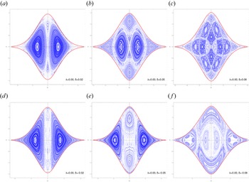
 . The Poincaré surfaces of section are given in figure 3. Figure 3(a–c) corresponds to ${\mathcal {H}}=E_0=V_{\max }$
 and figure 3(d–f) corresponds to $E_0>V_{\max }$
 . We observe that increasing $\lambda$
 induces trapping of the phase space orbits in the latter case.

Figure 3. Poincaré surface of section $Q_2 = 0$ for $\delta _1 =0.9$
 , $\delta _2=0.09$
 , $\delta = \delta _3-\delta _2=0$
 , $\kappa =1$
 , $E_0=V_{\max }$
 (a–c) and $E_0>V_{\max }$
 (d–f) showing the influence of $\lambda$
 on escape dynamics.
5.2.2 Nonintegrable case and chaotic dynamics
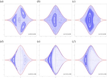
In the generic case $\delta _2\neq \delta _3$ , which corresponds to an anisotropic distribution function, the rotational symmetry of the potential is lost and the second integral of motion no longer exists. The loss of integrability results in the breakup of invariant tori and the subsequent emergence of islands of stability and chaotic regions in the Poincaré surfaces of section (See figure 4). As a result, the magnetic and the electric field fluctuations may be either periodic/quasiperiodic, if the initial conditions correspond to periodic/quasiperiodic trajectories in the phase space, or chaotic if the initial conditions fall into chaotic regions. As it can be deduced from figure 4, the breakup of the invariant tori and the extent of the chaotic region depends on the distribution function anisotropy in the $p_y\unicode{x2013} p_z$
 plane, which is quantified by the parameter $\delta =\delta _3-\delta _2$
 . Increasing the absolute value of $\delta$
 results in less organized phase-space configurations, with a large number of islands and extended chaotic regions.

Figure 4. Poincaré surface of section $Q_2 = 0$ for various values of the parameter $\delta = \delta _3-\delta _2\neq 0$
 (nonintegrable case). The emergence of chaotic regions is observed while $|\delta |$
 increases.
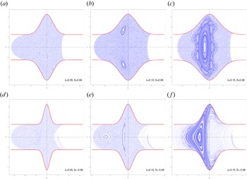
Regarding the qualitative influence of the Coriolis coupling parameter (Beltrami parameter), we notice a drastic reduction in the number of islands as $\lambda$ increases (figure 5). More specifically, as $\lambda$
 increases from $0.00$
 to $0.15$
 the phase-space trajectories are progressively organized into fewer, larger islands surrounded by a chaotic region, up to a point where a single extended island is formed. For the case $\delta >0$
 this island covers an extended region of the Poincaré surface of section that contains the origin $(Q_1,P_1)=(0,0)$
 ; thus for sufficiently small initial conditions the trajectories are stable and regular. Therefore, it can be inferred that the current density due to electrons can induce a regularization of the magnetic field dynamics and consequently a regularization of the bipolar electric field structures.

Figure 5. Poincaré surface of section $Q_2 = 0$ of the nonintegrable system for various values of the parameter $\lambda$
 and $E_0=V_{\max}$
 .
.
In terms of the escape dynamics, we observe that $\lambda$ plays a significant role in the confinement of the phase space trajectories when $E_0>V_{\max }$
 , as shown in figure 6. This was also seen in the case in the integrable system. As $\lambda$
 is increased from $0.05$
 to $0.15$
 , phase space trajectories starting from a specific region close to the origin $(Q_1,P_1)=(0,0)$
 on $Q_2=0$
 , occupy a progressively smaller region of the phase space and islands of stability are formed. For instance, when $\lambda =0.15$
 , an extended island that encloses the origin and is surrounded by a chain of smaller ones is formed, meaning that orbits originating from the vicinity of the origin will remain confined and regular. Similar findings have been reported for a rotating Hénon–Heiles system (Henon & Heiles Reference Henon and Heiles1964), which has been studied in Salas et al. (Reference Salas, Lanchares, Iñarrea and Farrelly2022). This represents another stabilization effect of $\lambda$
 , with the first one having been discussed in the previous subsection, which was about the change of the stability of the equilibrium point in the case of positive electrostatic potential, i.e. $\delta _1<0$
 .
.

Figure 6. Poincaré surface of section $Q_2 = 0$ of the nonintegrable system for various values of the parameter $\lambda$
 and $E_0>V_{\max}$
 .
.
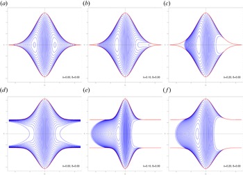
Closing this section we present two characteristic equilibria with multiple bipolar field structures in figure 7. In the first case the distribution function is gyrotropic and thus the magnetic field is integrable resulting in periodic pulses. The second corresponds to an asymmetric distribution function ($\delta _2\neq \delta _3$ ), and nonintegrable magnetic field resulting in pulses with irregular spatial distribution and amplitudes. In both cases $E_0=1.05\,V_{\max }$
 and $\lambda =0.1$
 so there is Coriolis trapping of the escaping trajectories. It has been verified that those structures emerge in positions associated with steep magnetic field gradients. Furthermore, the characteristic length scale of the pulses is determined by the distribution function parameters $\delta _1$
 , $\delta _2$
 and $\delta _3$
 and depend also on the initial conditions. The smallest structures we were able to construct have characteristic length scales of the order $0.1 \ell _i$
 .
.

Figure 7. Bipolar electric field pulses with negative electrostatic potential in the integrable (a) and the nonintegrable case (b). In the former case the pulses are periodic, while in the latter, they are irregular since the initial conditions correspond to a chaotic trajectory of the Hamiltonian system (4.27)–(4.30).
6 Harmonic oscillator potential: an inverse equilibrium problem
In the previous section we implemented the direct equilibrium construction where the pseudopotential is determined upon defining the ion distribution function. However, (4.17) can be seen as an integral equation for determining the function $g(\,p_y,p_z)$ in the expression for the distribution function, for a known pseudopotential $V(Q_1.Q_2)$
 . For example, we may choose a pseudopotential that enables the calculation of analytic solutions for the scalar and vector potentials and then solve the integral equation (4.17) for $g(\,p_y,p_z)$
 . In order to obtain a wave-like solution let us adopt a two-dimensional (2-D) anisotropic harmonic oscillator potential of the form

where $V_0$ , $\omega _1$
 and $\omega _2$
 are real constants. In this case the canonical Hamiltonian system (4.27)–(4.30) can be written in terms of the generalized coordinates $Q_1$
 , $Q_2$
 as
as


The system of (6.2)–(6.3) possesses the following analytic solution:


where $\eta _{1,2,3,4}$ are given in Appendix A and $c_i$
 , $i=1,\ldots,4$
 are arbitrary constants that are determined by the initial conditions imposed on the canonical variables $(Q_1,Q_2,P_1,P_2)$
 . The canonical momenta $P_1$
 , $P_2$
 can be easily derived from the definitions (4.23) and (6.4), (6.5).
Therefore, as is elementary, the Hamiltonian system with a 2-D anisotropic harmonic oscillator potential is integrable and solvable, although the angular momentum ${\mathcal {L}}$ is not conserved for $\omega _1\neq \omega _2$
 . Obviously, the Hamiltonian ${\mathcal {H}}$
 remains an integral of motion. If the oscillators were uncoupled ($\lambda =0$
 ), the Hamiltonian would be diagonal, and the energy stored in one of the degrees of freedom, ${\mathcal {H}}_1 = P_1^2/2+\omega _1^2 Q_1^2/2$
 , would be a second integral of motion. However, for $\lambda \neq 0$
 , the Hamiltonian is seemingly non-separable, and the second integral of motion is not directly apparent. Nonetheless, because the system is linear it must be transformable into one of the normal forms for linear systems (Moser Reference Moser1958) by a linear canonical transformation $(Q_1,Q_2,P_1,P_2)\rightarrow (\tilde {Q}_1,\tilde {Q}_2,\tilde {P}_1,\tilde {P}_2)$
 . If the system is stable, this amounts to a transformation to action-angle variables where the Hamiltonian is the sum of uncoupled oscillators. This separable form of the Hamiltonian reveals the second integral of motion. Specifically, by employing the canonical transformation presented in Appendix A ((A10)–(A13a,b)), we can show that in the stable case, the Hamiltonian takes the form

where, $\sigma _i\in \{\pm 1\}$ denotes the signature of the modes with frequencies $\zeta _i$
 . In Appendix A we show that $\sigma _1=-1$
 , thus $\zeta _1=\zeta _-$
 corresponds to a negative energy mode. Due to the large parameter space, we will not explore this further here and instead focus on the inverse equilibrium problem.
With the pseudopotential (6.1) the integral equation (4.17) reads

Whenever the right-hand side of (6.7) can be written as a polynomial of $Q_1$ and $Q_2$
 then there is a quite expedient method to compute the kernel $g(\,p_y,p_z)$
 and consequently the distribution function $f(H,p_y,p_z)$
 , using Hermite polynomials (see Channell Reference Channell1976; Allanson et al. Reference Allanson, Neukirch, Troscheit and Wilson2016a). The right-hand side of (6.7) can be expressed as a polynomial either if $\kappa$
 is a positive integer (or zero in the cold electron limit) or if $\omega _1^2 Q_1^2/2 + \omega _2^2 Q_2^2/2 < V_0$
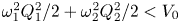 since in that case its Taylor series is convergent. In both cases, using the following relation (Channell Reference Channell1976):

where $H_{n}(x)$ is the $n$
 th-order Hermite polynomial defined by

Equation (6.7) can be expanded as follows:

Since the Hermite polynomials satisfy the following orthogonality conditions:

it is appropriate to expand the kernel $g(\,p_y,p_z)$ using a Hermite polynomial basis, i.e.

Inserting (6.12) into (6.10) and using the orthogonality of Hermite polynomials (6.11) we are left with

thus, the only non-vanishing coefficients $c_{nm}$ in the expansion (6.12) are

In addition, we have shown that (see (4.14), (4.15) and (4.17)) the electrostatic potential is given by

thus, for the anisotropic harmonic oscillator pseudopotential (6.1), $\varPhi$ reads as follows:

Consequently, the equilibrium distribution function is

As examples, consider two special cases: first, the cold electron limit, i.e. $\kappa =0$ , which implies $\varPhi =0$
 (strong neutrality); and second, the case $\kappa =1$
 . In the former case, which has been considered also in Channell (Reference Channell1976) (for the isotropic oscillator potential) the equilibrium distribution function reads as

The positivity of the distribution function is ensured if $V_0>\omega _1^2+\omega _2^2$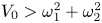 . In the latter case ($\kappa =1$
 ) the equilibrium distribution function is given by

where

One can find regions in the parameter space $(V_0,\omega _1,\omega _2)$ , in which the distribution function is positively defined.
7 Conclusion
We calculated equilibrium solutions to the hybrid Vlasov–Maxwell model with kinetic ions and massless fluid electrons by solving an inhomogeneous Beltrami equation, where the inhomogeneous term is the kinetic ion current density. To this end, we used the quasineutrality condition to express the electrostatic potential in terms of the vector potential components, instead of assuming strong neutrality to allow the emergence of large amplitude electric field structures due to fluctuations of the magnetic field. Then, we studied the Hamiltonian dynamics of the magnetic field equations and found that fluctuations are regular for ion distribution functions characterized by rotational symmetry in the $p_y\unicode{x2013} p_z$ plane, but can become chaotic for asymmetric ones. We have shown that the magnetic field equations constitute a Hamiltonian system and we have used Poincaré maps to show the existence of periodic, quasiperiodic and chaotic trajectories in phase-space, indicating that magnetic and electric field fluctuations can be either ordered or chaotic, depending on the initial conditions for the magnetic field and vector potential components. The electron current density affects the dynamics of the Hamiltonian system by altering the structure of the phase-space and the escape dynamics of the orbits through a Coriolis-like coupling between the generalized coordinates and the conjugate momenta. We observed that increasing electron current density progressively organizes phase space trajectories into large islands of stability and can induce the trapping of escaping phase-space orbits. The stabilizing effect of the electron current density was also ascertained upon performing a stability analysis of the equilibrium point. Upon increasing $\lambda$
 , the orbits in a neighbourhood of the equilibrium point can be stabilized even for positive electrostatic potentials. In this case, the electrostatic potential is modulated by the magnetic field fluctuations, enabling ion trapping. Finally, we provided an inverse equilibrium calculation where we computed the vector potential components and the ion distribution function by defining the pseudopotential of the Hamiltonian magnetic field dynamics. The particular choice of pseudopotential function results in a rotating, 2-D, harmonic oscillator Hamiltonian which is integrable and solvable. The distribution function is constructed assuming a multiplicative separability in $p_y$
 and $p_z$
 and using a Hermite expansion method. In future work, we plan to investigate the properties of Hamiltonian systems emerging in kinetic equilibrium problems, including the study of translationally symmetric plasmas, deviations from quasineutrality, and the existence of multiple ion species with fluid and kinetic components (e.g. Kaltsas, Throumoulopoulos & Morrison Reference Kaltsas, Throumoulopoulos and Morrison2021). In these frameworks the development of models capable of describing bipolar structures that closely resemble those observed by the MMS mission will be pursued.
Acknowledgements
The authors would like to thank A. Tenerani for providing insightful comments that helped to improve the manuscript.
Editor T. Passot thanks the referees for their advice in evaluating this article.
Funding
This work has received funding from the National Fusion Programme of the Hellenic Republic – General Secretariat for Research and Innovation. P.J.M. was supported by the US Department of Energy contract no. DE-FG05-80ET-53088.
Declaration of interests
The authors report no conflict of interest.
Appendix A. Normal form Hamiltonian
In § 4 we found a canonical Hamiltonian that describes the magnetic field dynamics in 1-D hybrid Vlasov equilibria. Upon Taylor expanding the potential of this Hamiltonian we obtain

where $V_0 = V(\xi _e)$ and
and

Hereafter the overbar will be dropped. For the pseudopotential (5.6), $V_1$ and $V_2$
 are given by (5.13a,b) and $U(Q_1,Q_2)$
 represents the $\mathcal{O}(Q^3)$
 terms. For the harmonic oscillator potential (6.1) in § 6, $V_1=\omega _1^2$
 , $V_2=\omega _2^2$
 and $U=0$
 .
.
To assess the stability of the fixed point $\xi _e=(0,0,0,0)$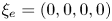 and in order to write the Hamiltonians in normal, diagonal form, we have to calculate the Hamiltonian spectrum of the equilibrium point. The eigenvalues of the stability matrix at $\xi _e$
 are given by

Here,


where $D^2{\mathcal {H}}(\xi _e)$ is the Hessian of the Hamiltonian ${\mathcal {H}}$
 evaluated at the equilibrium point $\xi _e$
 ,
,

The eigenvalues (A3) are thus given by

and the two frequencies are

Following Morrison & Kotschenreuther (Reference Morrison and Kotschenreuther1990), in the stable case ($\zeta _\pm \in \mathbb {R}$ ), we can diagonalize the Hamiltonian through a linear canonical transformation introducing the following generating function of type-2:

with

In the isotropic case $V_1=V_2$ we have

The new coordinates and momenta can be computed by the following equations:

Then, substituting the new variables in ${\mathcal {H}}$ we obtain a Hamiltonian of the form

which has the standard form for a negative energy mode that corresponds to the frequency $\zeta _1:=\zeta _-$ .
.


 Open access