


Introduction
In recent years, digital radar waveforms based on orthogonal frequency-division multiplexing (OFDM) have attracted a lot of attention in research and industry. Some of the reasons are the adaptability of the waveform, the ability to easily generate orthogonal transmit (Tx) signals required for multiple-input multiple-output (MIMO) systems [Reference Sturm, Sit, Braun and Zwick1–Reference Hwang, Yang, Wu, Li and Li3], and last but not least their suitability for joint communication and sensing applications [Reference Giroto de Oliveira, Nuss, Alabd, Diewald, Pauli and Zwick4, Reference Baquero Barneto, Riihonen, Turunen, Anttila, Fleischer, Stadius, Ryynänen and Valkama5]. Besides theoretical studies, several demonstrators have been built over the years, e.g., in [Reference Sit, Nuss and Zwick6] and [Reference Sanson, Tome, Castanheira, Gameiro and Monteiro7], which could prove some of the advantages mentioned, but in most cases also showed the limitations and challenges that have to be solved when building digital radars [Reference Schweizer, Grathwohl, Rossi, Hinz, Knill, Stephany, Ng and Waldschmidt8].
If a high range resolution has to be achieved, the classical OFDM approach covering the complete bandwidth digitally has a big disadvantage. In this case, high sampling rates and hence fast digital-to-analog (DAC) and analog-to-digital converters (ADC) are needed. To overcome this challenging requirement, several extensions of the conventional OFDM radar scheme have been proposed in literature. They all aim to increase the overall bandwidth covered during the radar measurements without changing the sampling rates. Hence, the range resolution can be improved. The first approaches dealing with this problem can be found in [Reference Huo, Deng, Liu, Jiang and Mao9] and [Reference Lellouch, Mishra and Inggs10]. Both methods increase the carrier frequency between consecutive blocks of multiple OFDM symbols either stepwise or according to a Costas pattern. However, their performance decreases significantly in case of moving targets, since the phase between the modulation symbols at different carrier frequencies changes too much due to their long durations and the Doppler shift.
One approach that does not degrade dramatically with moving targets was published in [Reference Pfeffer, Feger and Stelzer11] under the name stepped-carrier OFDM radar. There, the carrier frequency is increased by the signal bandwidth for consecutive OFDM symbols instead of only after blocks of multiple symbols. However, overlapping subcarriers are required for phase correction, which can lead to errors, particularly in the case of a poor signal-to-noise ratio. For this reason, the method including the associated signal processing scheme was further optimized in [Reference Schweizer, Knill, Schindler and Waldschmidt12] and [Reference Schweizer, Schindler, Knill, Hasch and Waldschmidt13] and the hardware requirements and effects were examined in [Reference Schweizer, Schindler, Knilll, Hasch and Waldschmidt14]. The disadvantage of this method is that the time interval between successive OFDM subsymbols at the same carrier frequency increases by the number of steps. Furthermore, there are additional pauses required due to the settling time of the local oscillator (LO) after the frequency jumps. Both effects lead to a significantly reduced unambiguous velocity. This can be circumvented by using a second LO [Reference Schindler, Schweizer, Knill, Hasch and Waldschmidt15] to allow one of the oscillators to settle while the other is active, but this increases the hardware complexity and the two LOs must be precisely matched.
Another method in [Reference Schindler, Schweizer, Knill, Hasch and Waldschmidt16] uses a linearly increasing frequency ramp as carrier for narrowband OFDM symbols instead of frequency steps. However, in the range-Doppler map after the signal processing of this scheme, the broad target peaks in range direction resulting from the narrow bandwidth of the original OFDM signal are tilted from the range direction toward a diagonal range-Doppler direction. These diagonally oriented broad peaks in the range-Doppler map can still mask closely separated weaker targets and thus, the resolution remains effectively unchanged in this dimension. Furthermore, instead of a stepwise or continuous increase, a combination of pseudo-random carrier frequencies with blocks of OFDM symbols of different number and bandwidth can also be used, as shown in [Reference Knill, Schweizer, Sparrer, Roos, Fischer and Waldschmidt17]. In this case, however, the range and velocity of the targets can no longer be estimated using simple discrete Fourier transforms (DFTs), but more computationally intensive optimization algorithms have to be used instead.
An alternative approach is the frequency comb OFDM radar scheme first published in [Reference Nuss, Mayer, Marahrens and Zwick18]. There, the analog signal bandwidth is increased by upconverting a narrowband OFDM signal with a frequency comb whose carrier spacing is equivalent to the OFDM bandwidth. Due to the narrowband OFDM baseband signal, the DAC can operate at a low sampling rate compared to the ultimately transmitted signal. Furthermore, the ADC in the receiver also operates at the same low sampling rate. To retain the relevant channel information of the wideband receive (Rx) signal nonetheless, a second frequency comb is used at the receiver for the downconversion. To avoid overlapping between the subcarriers during the downconversion with the second comb, not all subcarriers in the Tx signal are utilized. The resulting gaps can be used at the Rx to shift in the orthogonal subcarriers of all subbands and all Tx channels. Hence, a common narrowband frequency band results that contains all actively used subcarriers of the wideband Rx signal. A big advantage of the scheme is the high unambiguous velocity that can be achieved since there are no pauses between consecutive OFDM symbols at the same carrier frequency.
To verify the capabilities of the frequency comb OFDM radar scheme and to prove that direction of arrival (DoA) estimation based on spectral subcarrier interleaving described in [Reference Sturm, Sit, Braun and Zwick1] using a MIMO setup is still possible, a suitable demonstrator is required. In addition, there are specific demands on this proof-of-concept demonstrator since the combination of the narrowband OFDM subbands requires strict phase coherency among the comb frequencies as well as attention on the effects when mixing two broadband signals. In the following such a demonstrator is presented that is capable of performing verification measurements with the frequency comb MIMO OFDM radar scheme. In comparison to [Reference Nuss, Mayer, Marahrens and Zwick18], where only single-input single-output (SISO) measurements were shown and [Reference Nuss, Giroto de Oliveira and Zwick19], which presented different MIMO allocation schemes and their processing, the current paper focuses on the MIMO demonstrator itself showing the considerations made in the design phase, the challenges that had to be solved therein, and the results that could be achieved with the demonstrator.
The remainder of this article is organized as follows. Section ‘Frequency comb OFDM radar’ summarizes the signal generation and processing of the scheme. In Section ‘Demonstrator setup’, the components of the demonstrator are described in detail and in Section ‘Radar measurements’ measurements results achieved by the demonstrator are presented before this article is concluded in Section ‘Conclusion’.
Frequency comb OFDM radar
According to [Reference Nuss, Giroto de Oliveira and Zwick20] and [Reference Nuss21], the Tx signal is divided into a sequence of frames, each with a length of T obs and consisting of M OFDM symbols. Each of these symbols with the duration T 0 in turn consists of N subcarriers spanning in total a signal bandwidth of B. However, not all of the subcarriers have to be active. In front of each OFDM symbol, a cyclic prefix (CP) with the duration T cp = N cp ⋅ T s with T s being the sampling time is inserted. Thus, the effective symbol duration is increased to T = T 0 + T cp. Except otherwise stated, the CP is omitted in the following equations for simplicity. Hence, the complex baseband signal of Tx channel p after DAC conversion and low-pass filtering can be described by

Here, ${p = 0,\; \, \dots ,\; \, P - 1}$ is the index of the Tx channels belonging to the respective antennas, ${n = 0,\; \, \dots ,\; \, N-1}$
 is the subcarrier index, Δf = 1/T 0 = B/N the subcarrier spacing and Xp holds the payload data. According to [Reference Nuss, Giroto de Oliveira and Zwick19], the payload data can be written in matrix notation as

if the active subcarriers are allocated in an equidistant way to the P Tx channels. ${\cal A}$ is the modulation alphabet, e.g., QPSK. Equation (2) shows that only every (P L)th subcarrier is used. In comparison to the SISO scheme in [Reference Nuss, Mayer, Marahrens and Zwick18], the distance between the active subcarriers is increased by a factor of P to account for the number of simultaneously active transmitters. In addition, the factor L is needed to provide gaps in the spectrum that can be used in the baseband of the receiver to combine the subcarriers of all subbands in a narrow frequency band of bandwidth B without mutual interference.
The narrowband OFDM signal x p(t) is then upconverted in the transmitter with the frequency comb [Reference Nuss, Mayer, Marahrens and Zwick18]

Here, the spacing of the L comb frequencies is identical to the signal bandwidth B and f c,0 is the lowest comb frequency.
The upconverted signals

are transmitted via the P Tx antennas, reflected at the targets and received at the Q Rx antennas.
For a single point target, the Rx signal at antenna q is given as

τ q,p(t) = (R 0,p + R 0,q − (v p + v q)t)/c 0 is the time variant delay between Tx antenna p, the point target and Rx antenna q. R 0,p and R 0,q are the initial distances between the two antennas and the target and v p and v q are the relative radial velocities. α q,p is the attenuation factor calculated by the radar equation and c 0 is the speed of light. For simplicity, noise has been omitted in (5).
The receive signal r q(t) is downconverted with a second frequency comb [Reference Nuss, Mayer, Marahrens and Zwick18]

whose spacing between the comb frequencies is (B − Δf), which is slightly smaller compared to the spacing of B in (3). Consequently, all subbands are superimposed in a common frequency band of bandwidth B, but due to the differences in the Tx and Rx combs no overlapping occurs, since the subcarriers of the different subbands are shifted into the gaps of the original OFDM spectrum. In addition, their orthogonality is maintained in such a way that they can be separated after the digitalization and assigned to their individual subbands and transmitters. Finally, the spectra of the broadband receive signals can be reconstructed digitally for each of the P ⋅ Q virtual channels resulting in

Here, the index ${n = 0,\; \, \dots ,\; \, N L - 1}$ covers all subcarriers of the combined spectra. For all exponential terms except the one containing ϕ q,p, the approximations R 0,p ≈ R 0,q ≈ R 0, v p ≈ v q ≈ v and f c,0 ≫ B have been used. For ϕ q,p = −2πf c,0(R 0,p + R 0,q)/c 0, the small range differences can not be neglected since they are used to estimate the DoA. f D = 2 f c,0v/c 0 is the Doppler shift for a moving target and the center frequency related to the broadband signal is f c = f c,0 + ((L − 1)/2)B. For the sake of simplicity, range migration and inter-carrier interference have been neglected in the mathematical expression in (7), but are accounted for in the simulations and measurements.
Next, the payload data Xp is removed by an elementwise division,

to get the channel information. The range is then estimated by an inverse discrete Fourier transform (IDFT) along the subcarriers of each OFDM symbol,

followed by an DFT along the rows of (9),

to extract the Doppler information. Finally, the DoA is estimated via a simple Fourier beamforming [Reference Nuss, Sit, Fennel, Mayer, Mahler and Zwick22].
Demonstrator setup
To demonstrate the functionality of the frequency comb OFDM radar scheme capable of estimating the range, velocity and azimuth angle of real targets, a MIMO-enabled demonstrator was designed and built. This includes two MIMO boards with four channels each for the up- and donwconversion with the frequency combs as well as two modules generating the comb frequencies for the transmitter and receiver. In addition, software defined radios (SDRs) of type USRP X310 from Ettus Research were used to generate and receive the necessary OFDM signals, as well as to generate the sine waves from which the comb frequencies are derived.
Frequency comb generation
For the frequency combs, there are two major requirements that have to be fulfilled according to the experiments and analysis made with the previous SISO demonstrator in [Reference Nuss, Mayer, Marahrens and Zwick18]. First of all, the comb frequencies have to be phase coherent during the complete measurement cycle. This includes the observation time of the radar measurement itself but also the calibration phase before which is necessary to compensate for the transfer functions of the SDRs and front-ends as well as for starting phases of the comb frequencies. And second, initial experiments showed that feeding the available passive mixers with two broadband signals, the OFDM and the comb signal, would result in strong intermodulation products which would reduce the dynamic range. Thus, the OFDM signals are up- and downconverted individually with the single comb frequencies and then combined afterwards. To achieve good phase coherency, all comb frequencies have to be derived from a single source. The block diagram of the circuit specifically developed for this purpose which simultaneously delivers the single comb frequencies at the output ports is shown in Fig. 1.

Figure 1. Block diagram of the comb generation circuit, starting with the sinusoidal signal at the SDR output which is used to generate a frequency comb in the baseband. After separation of the comb frequencies with the help of a diplexer they are upconverted in an image reject mixer to the RF. The frequencies marked in black are for the Tx case and the ones marked in red for the Rx case.
At the beginning, a sinusoidal reference signal is generated digitally in one of the SDRs with a frequency of either B/4 in the Tx or (B − Δf)/4 in the Rx case. The reduction of the frequency by a factor of four is necessary to fulfill the Nyquist criterion since the maximum sampling rate of the SDRs is limited to f s = B = 100 MHz. In particular in the Rx case, the image frequencies could not be suppressed sufficiently if the reference signal would be at twice the chosen frequency. Afterwards, the frequency is doubled in a frequency multiplier to compensate for the previously described reduction. The output signal is then again doubled in frequency and used as LO signal at a mixer to upconvert the intermediate signal at f = B/2 resulting in f = {1/2, 3/2}B for the Tx case. These two frequencies are then separated in a duplexer since the comb frequencies are needed individually. To upconvert them from baseband to the radio frequency (RF), four image reject mixers build up of quadrature hybrid couplers and IQ mixers were used. Depending on which input ports of the couplers are used, the four different comb frequencies shown on the right in Fig. 1 are generated. The corresponding realization of the circuit can be seen in Fig. 2.

Figure 2. Comb generation board where the four comb frequencies are derived from a single source to achieve phase coherency (figure based on [Reference Nuss21]).
The reference signal coming from an SDR is fed in on the left side followed by the comb generation in the baseband. In the middle of the right side, the LO signal to upconvert the baseband comb frequencies is fed in next to the outputs of the final comb frequencies. The measured output levels of these signals as well as adjacent spurious emissions are visible in Fig. 3 and listed in Table 1.
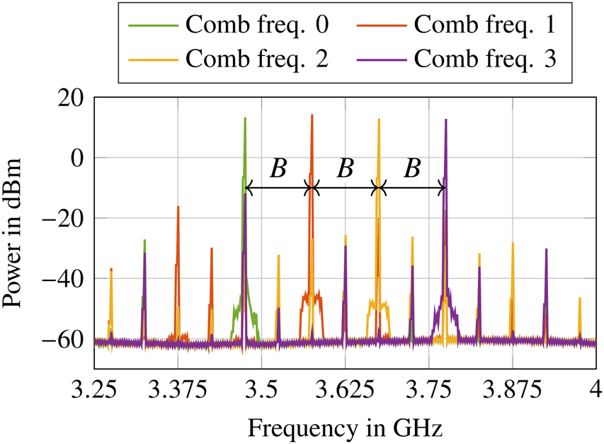
Figure 3. Separately measured and superimposed spectra of the four output channels of the comb generation board (figure based on [Reference Nuss21]).
Table 1. Performance of the comb generation board

An alternative method to generate the required frequency combs and to subsequently upconvert the narrowband OFDM signals is presented in [Reference Quint, Nuss, Diewald and Zwick23].
Generation of the broadband OFDM signal
On the Tx side, a circuit was needed to generate the broadband Tx signals by upconverting the narrowband OFDM signals with the frequency combs. However, as test measurements showed, the direct mixing of the OFDM signal with the frequency comb in a single passive mixer resulted in very strong intermodulation products which significantly reduced the dynamic range of the radar. For this reason, a concept was chosen in which the OFDM signal is split in a power divider and then mixed separately with the individual comb frequencies. The resulting output signals are then recombined to produce the desired broadband signal.
For the DoA estimation, a MIMO setup with multiple Tx and Rx channels was required. Due to the large number of L ⋅ P mixers and the according number of necessary supply and transmission lines, a compact printed circuit board (PCB) was designed instead of using connectorized components. On this PCB, the OFDM signals fed in are mixed in parallel in P = 4 Tx channels with L = 4 comb frequencies and the resulting output signals are recombined and amplified. To reduce the number of connectors and the demands on the mixers, the OFDM signals are already upconverted to an intermediate frequency (IF) of f IF = 2.4 GHz inside the SDRs. Fig. 4 shows the realization of this board built in a metallic housing, whereas Fig. 5 presents the spectra of the four enhanced OFDM signals at the output ports.

Figure 4. RF board for the upconversion of the narrowband OFDM signals with the four comb frequencies (figure based on [Reference Nuss21]).

Figure 5. Spectra of the four Tx signals at the output ports of the upconversion board (figure based on [Reference Nuss21]).
Here, the L = 4 combined subbands and the rectangular shape of the OFDM spectrum with almost no intermodulation products in adjacent bands can clearly be seen.
Due to the different lengths of the transmission lines between the LO ports and the mixers of the four channels, the output power is decreasing from channel number 0 to 3. The Rx board is built very similar to the Tx PCB, except for the orientation of the amplifiers and some additional filters in the IF stage.
MIMO antenna
To estimate the DoA, a MIMO antenna consisting of P = 4 Tx and Q = 4 Rx antennas is used, as shown in Fig. 6.

Figure 6. MIMO antenna with four Tx channels (bottom) and four Rx channels (top).
Here, the number of antennas is limited by the number of usable SDR channels which in turn is restricted by the maximum data rate between the SDRs and the host PC. The Tx antennas are spaced by d Tx = 2λ c and the Rx antennas by d Rx = λ c/2. Together they form a virtual array that consist of P ⋅ Q = 16 elements with an equidistant spacing of d virt = λ c/2. Thus, an unambiguous azimuth angle of $180^\circ$ can be achieved.
Since the antenna elements have to meet the required total bandwidth of B tot = L ⋅ B = 400 MHz at a center frequency of f c = 6.025 GHz, no simple patch antennas could be used. Thus, the patches were supplemented with two laterally attached parasitic elements with a slightly different resonance frequency. The resulting effects can be seen quite well in the input return loss characteristic in Fig. 7 showing two adjacent dips that belong to the two resonance frequencies.
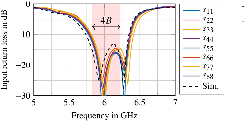
Figure 7. Measured input return loss of the Tx (1–4) and Rx (5–8) antenna elements in the array. As comparison, the simulated curve of a single element is given.
In addition, stepped metal barriers were inserted between the two arrays to suppress the mutual coupling. The MIMO antenna shown is based on a similar setup published in [Reference Nuss, Sit, Fennel, Mayer, Mahler and Zwick22]. The outer metal walls are necessary to tilt the antenna beam back to the broadside of the array. Accordingly, the beam width is reduced in elevation but maintained in azimuth direction. Due to the metal barriers, the coupling between the Tx and Rx elements can be limited to almost below −60 dB in the occupied frequency band as Fig. 8 shows.
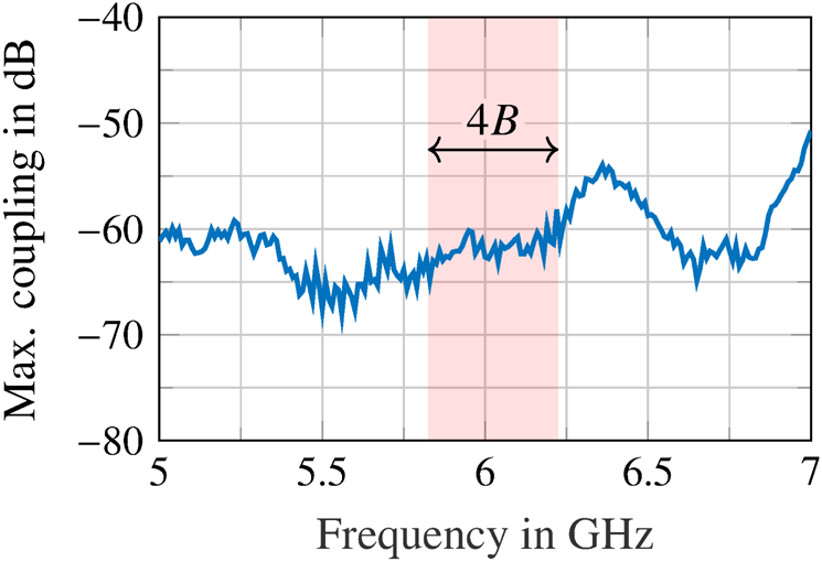
Figure 8. Maximum coupling between any of the Tx and Rx antenna elements.
This is in particular advantageous for digital radar systems where the transmitter and receiver are covering simultaneously the complete radar bandwidth and thus, a suppression of the directly coupled signal via filters or switches is not possible anymore.
Radar measurements
For the verification measurements, the previously described demonstrator was placed in an anechoic chamber. Due to the spatial limitations of this chamber, no real moving targets could be used. Thus, an analog radar target simulator (RTS) was set up which could add a Doppler shift to the reflected signal that is comparable or even higher than that of real objects.
Parameterization
The parameterization of the demonstrator essentially had to be based on the available hardware and the performance of the SDRs and the host PC. The latter two had a limited sampling and data rate and a limit on the available memory. For this reason, on the one hand, the bandwidth B was limited to 100 MHz, as specified in Table 2, and on the other hand, only the reception of about 400 000 IQ samples was possible which resulted in an observation time of T obs = 3.28 ms.
Table 2. Parameterization of the demonstrator
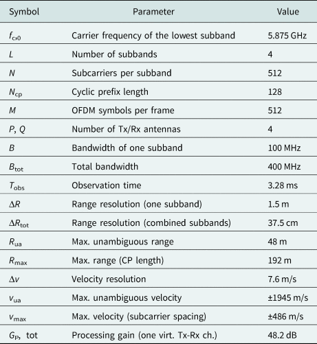
This restriction primarily affected the choice of the number of subcarriers N and the number of OFDM symbols M per measurement cycle, since their product determined the length of the OFDM frame. In addition, the samples of the CP had to be taken into account. Choosing N = M = 512 and N cp = N/4 resulted in a frame length of (N + N cp) ⋅ M = 327680. In this context, N could not be chosen too small, since the number of actively used subcarriers in the MIMO case was reduced to N/(L P). This also led to a reduction of the unambiguous range to

On the other hand, if N was chosen too high, the maximum tolerable velocity v max would have been significantly smaller. This in turn would have greatly impaired the proof that the method also works at very high relative velocities of the targets.
Due to the limitation of the maximum frame length, the achievable velocity resolution was also fixed to Δv = 7.6 m/s, since it is inversely proportional to the measurement duration T obs. In addition, the processing gain for one of the P ⋅ Q virtual Tx-Rx channels was $G_{\rm P, \, tot} = N M / P \ \hat = \ 48.2$ dB.
dB.
The number of Tx and Rx channels, P and Q, was limited by the data rate between the SDRs and the host PC as well as the available memory. The best behavior was shown for an even load on the connection resulting in P = Q = 4 considering the limitations. The MIMO antenna shown in Fig. 6 was also designed on this basis.
The choice of L = 4 is a compromise between the enlargement of the bandwidth and the hardware complexity, since an increase in the number of comb frequencies would have resulted in a larger number of mixers. By increasing the bandwidth by a factor of four, the theoretical range resolution could be improved from ΔR = 1.5 m of a single subband to ΔR tot = 37.5 cm when evaluating all subbands together.
Measurement setup
For verification measurements, the setup was placed in an anechoic chamber with a size of about 4.0 m × 6.5 m which was lined with absorbers. Since the chamber was too small to move real targets with high velocities, an analog RTS has been built which could realize very high Doppler shifts. There, the signal received by the RTS is downconverted by a first LO with f LO,1 = 5,025 GHz to an IF of 1 GHz, low-pass filtered and then upconverted with a slightly shifted second LO with f LO,2 = 5,025 GHz + f D. Afterwards, the signal is band-pass filtered to suppress the unwanted image and then re-transmitted in direction of the radar. Fig. 9 shows the view from the demonstrator into the anechoic chamber, which contained either two static corner reflectors, each with a radar cross-section of about 26 m2, or the RTS mentioned instead of the second corner.
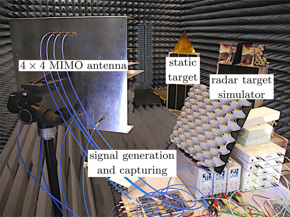
Figure 9. Measurement setup with the 4 × 4 MIMO antenna pointing toward a static corner reflector on the left and the antennas of the analog RTS on the right.
Calibration
At the beginning of each measurement series, a calibration had to be carried out in order to compensate both the amplitude and phase responses of the hardware and the internal delays. In addition, phase differences between the subbands within each MIMO channel and between the Tx and Rx channels were compensated for during the calibration. On the one hand, this was necessary to seamlessly combine the subbands and, on the other hand, to enable DoA estimation in the first place. For the calibration, the outputs of the Tx board were connected to a power combiner, which in turn was connected to a power divider via an attenuator. Its four outputs finally led to the inputs of the Rx board such that all Tx and Rx channels were connected with each other. Using the orthogonal MIMO signals, the relative amplitude and phase differences between the individual channels could be determined and consequently compensated for by an elementwise division of all further measured OFDM frames by the one captured during the calibration. The deviations resulting from the power divider and combiner themselves could be neglected compared to the effects of the other components. It also had to be noted that during the calibration and the later radar measurements the same cables were used to minimized the deviations between the actual and the reference measurement.
A comparison of Figs. 10a and 10b illustrates the effect of the calibration.

Figure 10. Range profile for the evaluation of a single Tx-Rx pair at 0 m/s for a scenario with a direct connection of the Tx and Rx channels (a) without and (b) with calibration.
For both measurements, the setup with the direct connection via combiner and divider was used and all channels were active simultaneously. Thus, ideally a single peak should be visible at R = 0 m and v = 0 m/s in the range profile of each Tx-Rx channel. However, as can exemplarily be seen in the uncalibrated case in Fig. 10a, the curves of the individual subbands already show distortions and different amplitudes. In addition, their maxima are not located at R = 0 m and phase jumps between adjacent subbands can occur. This explains the high sidelobe level after the combination of the subbands, resulting in a significantly lower dynamic range than in theory.
After the calibration, however, the individual peaks in Fig. 10b were clearly visible and the curves of all four subbands lay on top of each other neglecting noise. In addition, the sidelobes were significantly reduced and the dynamic range was almost 55 dB. Furthermore, a closer look at the main peaks on the right side clearly shows the improvement of the range resolution by a factor of four after the joint evaluation of all subbands.
Separation of two adjacent targets
The main goal of the frequency comb OFDM radar scheme is to increase the signal bandwidth in the radar channel and hence to improve the range resolution. To verify this property, two static corner reflectors were positioned in front of the radar, the first one in a distance of 2.6 m and the second one at 4.0 m, resulting in a distance of about 1.4 m between the two objects which is below the theoretical range resolution of a single subband. Thus, it was to be expected that if the individual subbands were evaluated separately, the two targets would not be separable from one another. Only the combination of the subbands according to the frequency comb-based approach made it possible to improve the resolution by a factor of L = 4 and consequently separate the two targets as can be seen in Fig. 11.

Figure 11. Range profile for a single Tx-Rx pair at 0 m/s for a scenario with two static targets that are about 1.4 m apart.
Targets with high velocities
In [Reference Nuss, Giroto de Oliveira and Zwick20], it was described that using the frequency comb OFDM radar scheme in conjunction with high velocities can lead to the occurrence of ghost targets due to the increasing loss of orthogonality between the subcarriers. According to Table 2, this effect is neglectable for targets at velocities below v max = ±486 m/s which can also be validated in Fig. 12a and 12b, where there is an emulated target with v = 200 m/s and v = 400 m/s, respectively. In both cases, no ghost targets are visible.

Figure 12. Measured range-Doppler plots of a single Tx-Rx pair with one static and one moving target with (a) v = 200 m/s, (b) v = 400 m/s, and (c) v = 1600 m/s. In case of high velocities, ghost targets occur due to inter-carrier interference.
If the velocity, however, is further increased, e.g., to v = 1600 m/s as demonstrated in Fig. 12c, ghost targets occur at

where v is the actual velocity of the target. ${x' \in {\mathbb Z}}$ has to be chosen in such a way that v g lies within the unambiguous velocity interval [ −v ua, v ua] [Reference Nuss21]. To avoid this effect, either an adaption of the MIMO subcarrier allocation scheme or a proper choice of the CP length is possible as described in [Reference Nuss, Giroto de Oliveira and Zwick20].
MIMO measurements
The MIMO setup with four Tx and four Rx antennas allows to perform 3-D radar measurements estimating the range, velocity and azimuth angle of targets. For a better visualization of the measurement data, only superimposed slices of the three-dimensional matrices have been plotted in Fig. 13. For the superposition, the two-dimensional range-azimuth plots taken at the velocities v = 0 m/s and v = [200, 400, 1600] m/s of the two targets have been summed. The peak at the azimuth angle $\varphi = -1^\circ$ represents the reflection from the static corner reflector and the peak at $\varphi = 15^\circ$
 originates from the RTS, which fits quite well to the real measurement setup shown in Fig. 9. As the targets can clearly be seen in all three subplots in Fig. 13 and no unexpected effects are visible, it can be concluded that the frequency comb OFDM radar scheme does not affect the results of the MIMO processing, which is identical to the conventional OFDM radar approach.

Figure 13. Measured range-azimuth plots with one static ($\varphi = -1^\circ$ ) and one moving target ($\varphi = 15^\circ$
 ) with (a) v = 200 m/s, (b) v = 400 m/s, and (c) v = 1600 m/s.
Conclusion
The frequency comb OFDM radar scheme enables the improvement of the range resolution without increasing the baseband sampling rate or the complexity of the signal processing. In addition, the high unambiguous velocity of the classical OFDM radar approach is retained. To validate both features and to prove that the scheme is still suitable for DoA estimation using MIMO, a proper demonstrator has been developed and set up. For the verification measurements the demonstrator was placed in an anechoic chamber where the separation of two closely spaced targets, the DoA estimation, and the predicted occurrence of ghost targets at high velocities could be shown successfully. In addition, the necessity of a calibration to eliminate phase and amplitude deviations between the comb frequencies and hence the subbands has been demonstrated.
Conflict of interest
The author(s) declare none.
 Benjamin Nuss received the B.Sc. and M.Sc. degrees in electrical engineering and information technology from the Karlsruhe Institute of Technology (KIT), Karlsruhe, Germany, in 2012 and 2015, respectively. In 2021, he received the Dr.-Ing. (Ph.D.E.E) degree from KIT and is currently working as a group leader for radar systems at the Institute of Radio Frequency Engineering and Electronics (IHE). The focus of his work is on the development of efficient future radar waveforms as well as on the design of joint communication and sensing systems. His current research interests include orthogonal frequency-division multiplexing based multiple-input multiple-output radar systems for future automotive and industrial applications.
 Lucas Giroto de Oliveira received the B.Sc. and M.Sc. degrees in electrical engineering with a major in electronic systems from the Federal University of Juiz de Fora (UFJF), Brazil, in 2017 and 2019, respectively. He is currently pursuing the Dr.-Ing. (Ph.D.E.E.) degree at the Institute of Radio Frequency Engineering and Electronics (IHE) of the Karlsruhe Institute of Technology (KIT), Germany. His research interests are in the areas of system design, signal processing, digital communication, and their applications to integrated radar sensing and communication systems and networks.
 Thomas Zwick received the Dipl.-Ing. (M.Sc.) and Dr.-Ing. (Ph.D.E.E.) degrees from the Universität Karlsruhe (TH), Germany, in 1994 and 1999, respectively. In October 2007, he became a Full Professor with the Karlsruhe Institute of Technology (KIT), Germany. He is currently the Director of the Institute of Radio Frequency Engineering and Electronics (IHE), KIT. His research topics include wave propagation, stochastic channel modeling, channel measurement techniques, material measurements, microwave techniques, millimeter-wave antenna design, wireless communication, and radar system design.


 Open access