


Impact Statement
Popping of the cork stopper sealing a champagne bottle unequivocally represents an appealing prototype of a daily-life event that offers a remarkably rich variety of physical phenomena at play. Here, these accompany the sudden opening of, in more general terms, a vessel partially filled with a pressurised liquid and dissolved gas (mostly carbon dioxide). Extending the detailed numerical investigation put forward to the situation of more complex geometries and/or different sealing devices having different material properties is an indicated task of further activities. The current focus on the involved gas dynamics, highly unsteady and supersonic albeit at relatively moderate Mach numbers, might already provide a better insight into the complex details, specifically the shock structures, of transitional ballistics in related but more extreme situations of engineering importance. The study is also viewed as a benchmark test for future experimental and numerical efforts, in particular the spatial/temporal resolution of the full fluid–structure interaction of a high-speed gas flow with a solid moving obstacle. We suggest further modelling activities to predict (amongst others) the impact of temperature variations on the initial pressure inside the bottle by virtue of the solubility of carbon dioxide and the limitations of the inviscid-flow model for such scenarios, given the subtle role of viscosity lurking.
1. Motivation and introduction
The quite recent experimental study by Reference Liger-Belair, Cordier and GeorgesLiger-Belair, Cordier, and Georges (2019), succeeding the pioneering ones by Reference Vollmer and MöllmannVollmer and Möllmann (2012), Reference Liger-Belair, Bourget, Cilindre, Pron and PolidoriLiger-Belair, Bourget, Cilindre, Pron, and Polidori (2013) and Reference Liger-Belair, Cordier, Honvault and CilindreLiger-Belair, Cordier, Honvault, and Cilindre (2017), discloses the surprisingly complex formation of an expanding gas jet, propelling the cork stopper out of a just opened champagne bottle, where the jet and the stopper generate the typical popping sound by the radiation of shock waves. This stimulated us to tackle the challenge of resolving this process numerically in due detail, notably, by resorting to the forerunner investigation by one of us (Reference WagnerWagner, 2021). It is the ultimate goal of this work to supplement the experimental findings with theoretical predictions based on high-resolution computations. To this end, a modelling focus is laid on the essential physical mechanisms while effects of subordinate importance, either at play on smaller temporal/spatial scales or such as spontaneous phase transition, are deliberately ignored.
Taking up a rigorous point of view sets the basis for a least-degenerate, sound mathematical description of the problem that combines the fields of gas dynamics, fluid–structure interaction and solid–solid friction. Simultaneously, viscous effects are found as insignificantly weak over the spatial and temporal gross resolution of the jet propagation. Emphasis is then laid on the prediction of the axisymmetric supersonic gas jet, mixing perfectly with the ambient air while forming a complex shock pattern including a Mach disc or so-called shock diamond (cf. Reference ReichenbachReichenbach, 1983). This forms just outside of the bottleneck when the jet-driven stopper is already sufficiently remote from the latter. While the compressed gas inside the bottleneck technically contains  ${\rm CO}_2$ gas and water vapour besides small traces of alcohol, the first partial pressure value is vastly larger than the other readings and the problem is therefore considered as a single-phase problem with a heat capacity ratio at atmospheric pressure and $T=-40\,^\circ$C of $\kappa _{\mathrm {CO}_2}\approx 1.337$ (NIST, 2023). The ambient air surrounding the bottle has a ratio of $\kappa _{air}\approx 1.401$ (Engineering Toolbox, 2023). The fact that the temperature of the system can fall below $-100\,^\circ$C and $\kappa _{\mathrm {CO}_2}$ increases faster with decreasing $T$ than $\kappa _{air}$ does, explains why the difference between their ratios in the region of the Mach disc is even smaller. Additionally, the total mass of air vastly exceeds the one of ${\rm CO}_2$, explaining the nearly instantaneous mixing of both gases. Both considerations allow the assumption of a single-phase gas with a constant heat capacity ratio of $\kappa =1.4$ obeying the ideal gas law. This alleviates the computational effort drastically while the (viscosity-affected) mixing process itself would not alter the results substantially. The fraction of time within which the process is simulated spans from the effective opening of the bottle, seen as instantaneously fast, to the decay of the Mach disc.
We concede that the entire neglect of both viscous forces and the co-existence and mixing of two gaseous phases appears doubtful in variety of possible scenarios. To name the most critical ones, these include the shearing flow through the very small gap as the stopper just passes the bottle opening, gross separation of boundary layers accompanied by vortex formation as well as partial freezing of the carbon dioxide ( ${\rm CO}_2$) during its sufficiently strong (isentropic) expansion, observed by Reference Liger-Belair, Cordier and GeorgesLiger-Belair et al. (2019). However, these simplifications are substantiated by dimensional reasoning based upon the geometrical and kinematic reference scales. Consequently, they are admissible as their local/sudden invalidity would not affect severely the simulated dynamics of the stopper and the shock structure elucidated on those scales and being at the centre of our attention.
The resulting inviscid-flow simulations are preferably built upon the well-established open-source software environment Clawpack (Clawpack Development Team, 2022; Reference LeVequeLeVeque, 2002; Reference Mandli, Ahmadia, Berger, Calhoun, George, Hadjimichael and LeVequeMandli et al., 2016), centred around the usual combination of Godunov's numerical finite-volume scheme and Roe's approximate Riemann solver for hyperbolic systems of equations. Special care is taken to facilitate the complete gas–stopper interaction in a fully implicit manner and the stage of stopper–bottleneck interaction initiating the release of the stopper. Therefore, our approach contrasts with the recent computational study by Reference Benidar, Georges, Kulkarni, Cordier and Liger-BelairBenidar, Georges, Kulkarni, Cordier, and Liger-Belair (2022), complementing the aforementioned motivating experimental work: these authors employ the widely used commercial flow simulation software package Ansys Fluent![]() to solve the fully Reynolds-averaged Navier–Stokes equations using turbulence closures but disregard that initial stage entirely. The present investigation, however, aims at resolving the coupled gas and stopper dynamics of the whole process in the greatest possible detail, where our focus is on the formation of the Mach disc. It might thereby set the basis for a discussion and, in turn, proper inclusion of the here neglected viscous effects in this and closely related situations. In order to establish a reliable model of its compression/expansion and friction, tribological tests with a cork potentially in use were carried out at AC2T research GmbH.
to solve the fully Reynolds-averaged Navier–Stokes equations using turbulence closures but disregard that initial stage entirely. The present investigation, however, aims at resolving the coupled gas and stopper dynamics of the whole process in the greatest possible detail, where our focus is on the formation of the Mach disc. It might thereby set the basis for a discussion and, in turn, proper inclusion of the here neglected viscous effects in this and closely related situations. In order to establish a reliable model of its compression/expansion and friction, tribological tests with a cork potentially in use were carried out at AC2T research GmbH.
The paper is organised as follows. At first, we argue the simplifications addressed above to set up the corresponding physical–mathematical model (§ 2). This comprises the description of the gas and air flow, its interaction with the propelled stopper, subject to the dry sliding friction with the bottle prior to its expansion outside of this. We then outline in due detail the incorporation of particular numerical strategies in Clawpack that succeed in the stable resolution of the fully coupled gas–stopper interaction and solid–solid sliding (§ 3). As the bedrock of our study, the discussion of the results (§ 4) is accompanied by their comparison with those available in the literature and addressed above (§ 4.3). Finally, an outlook towards potential further implications completes the study (§ 5).
The supplementary material and movies are available at https://doi.org/10.1017/flo.2023.34, which contains two simulation movies (movie 1 and movie 2) and additional information, primarily addressing the technically interested reader, named ‘supplementary technical details’ (comprising supplements A–D in the supplementary PDF). However, the paper is self-contained to the necessary extent without the latter.
2. Physical model and problem formulation
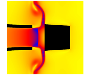
For what follows, we tacitly refer to the sketch in figure 1 throughout. The physical system considered consists of four parts, subject to a reasonable and self-consistent level of modelling abstraction, in good agreement with real-life observations (Reference Liger-Belair, Cordier and GeorgesLiger-Belair et al., 2019) and outlined in the following.

Figure 1. (a) Computational domain of coupled system bottleneck–stopper–gas (initial conditions); (b) detail of density plot at  $\tilde {t}=0.5$ ms; for colour levels of density see figure 9.
2.1 Basic assumptions
The physical system considered consists of four subsystems, representing the different materials involved. Its first part represents its boundary, formed by the perfectly rigid, impervious, axisymmetric, relatively slender bottleneck, typically made of glass. The accordingly impervious axisymmetric stopper made of cork forms the second. The third is given by the expanding gas, a solution of  ${\rm CO}_2$, slowly degassed by the liquid champagne and so accounting for its pressurisation prior to the opening of the bottle, air, alcohol and water vapour, which propels the stopper out of the bottle in the axial direction. It is confined by the surface of the contained champagne, during the process considered taken as a stationary, plane and impermeable boundary, and before the opening sealed by the stopper. For what follows, the bottleneck is then precisely defined as the void portion of the bottle between its opening and the liquid level. The initially quiescent ambient air represents the fourth subsystem. This, and the expanding gas, are taken as Newtonian ideal gases having constant specific heats, heat conductivities and dynamic viscosities (perfect gas), all of negligibly different magnitudes. Correspondingly, they form non-distinguishable phases, the mixing of which is entirely ignored, as are the temperature dependences of those quantities. Even though reasonable for the gas phase, this simplification admittedly disregards the phase transitions observed by Reference Liger-Belair, Cordier and GeorgesLiger-Belair et al. (2019).
The actual opening of the bottle effectively means the rapid overpowering of stiction (self-retention) between the stopper and the bottleneck, compressing the former radially, in favour of much lower sliding friction setting in. The so triggered force imbalance has the gas expand and starts the proper motion of the stopper. Here, this very first stage of the opening process is abstracted as instantaneous with respect to the resolved time scales. It thus provides the initial condition. Hence, the stopper is initially accelerated by the gas but decelerated by wall friction. The expanding gas remains contained in the bottle as long as the stopper has not entirely left the bottle. Simultaneously, it starts to move the outer air. Once it has left the orifice behind, it rapidly expands towards its original (decompressed) shape as it is pushed further by the now forming (under-expanded) gas jet and the thereby generated air flow. The gas and the air completely dissolve into one another, and the resulting flow and the motion of the stopper are presumed to remain axisymmetric.
We neglect the characteristic ‘dome’ of the stopper for a champagne bottle, which, in combination with the frustum at its base, gives it the characteristic mushroom-like appearance. However, this renders its discretisation unnecessarily complex whilst taking into account that the drag-increasing bumper would not alter substantially the fascinating flow patterns between the stopper and the bottle opening, tied in with the emergence of the Mach disc and fading out once the stopper is sufficiently remote from the opening. That surprisingly complex shock regime lies at the heart of our numerical analysis.
Before we specify the modelling of the four subsystems and their interactions, we summarise the essential assumptions and simplifications (i)–(vi):
(i) The ambient air and the pressurised gas mixture are indistinguishable single-phase ideal gases, characterised by constant (temperature- and pressure-independent) thermophysical properties (hence, the pressurised gas treated as air).
(ii) The bottleneck is beheld as a slender truncated cone, tapered towards the bottle opening, with sufficient accuracy. The mushroom-shaped cap of the stopper and the fastening wire cage (muselage) are both disregarded (as being irrelevant for the process under consideration).
(iii) The expanded (unloaded) stopper is also taken as a slender truncated cone, even though real sparkling wine corks are so-called agglomerated ones, composed of up to three rings of slightly different radii (Reference MargalitMargalit, 2012).
(iv) The cork used is typically modelled as a homogeneous and isotropic hyperelastic material of negligibly small lateral contraction: for this special case of an Ogden material model see Reference Sasso, Lattanzi, Farotti, Sarasini, Sergi, Tirillò and ManciniSasso et al. (2022), Reference Fernandes, Pascoal and Alves de SousaFernandes, Pascoal, and Alves de Sousa (2014) and references therein as well as Reference OgdenOgden (1997) and Reference DillDill (2006). Here, both the weak visco-elasticity usually found to be at play and the degradation of elasticity due to long-time ageing are ignored. Since the compressive reactive force the weakly tapered bottleneck exerts onto the stopper sliding along it appears to be much larger than all the other forces at play, the stopper can deform only radially while it remains rigid in the axial direction. Therefore, it assumes its original undeformed shape once its reversible decompression has stopped after a finite, properly defined relaxation time.
(v) We model the instantaneous expansion of the stopper by taking it as cylindrical when it has just left the bottle and on the basis of the estimated characteristic time scale at play rather than founding it more rigorously. This seems admissible given the relatively short duration of the expansion process.
(vi) We neglect any (unavoidable) leakage of gas out of the bottle as long as the stopper has not completely been released from it. That is, we may assume dry sliding (Coulomb) friction between the cork and the glass of the bottle (see Reference Fatima Vaz and FortesFatima Vaz & Fortes, 1998).
Furthermore, the following conventions prove sensible. Tildes indicate dimensional quantities while otherwise their non-dimensional form is used; the subscript  $0$ indicates the reference state of the quiescent ambient air; the subscripts $B$ and $C$ indicate the properties of, respectively, the bottleneck, including the pressurised gas initially at rest and provided by Reference Liger-Belair, Cordier and GeorgesLiger-Belair et al. (2019), and the cork stopper.
2.2 Geometry of bottleneck, unloaded stopper and computational domain
We introduce cylindrical coordinates  $\tilde {r}$ and $\tilde {z}$, radially from and along the axis of the bottle outwards from its opening, respectively. Let us first describe the two truncated cones representing the bottleneck and the fully relaxed stopper as inferred from figure 1. The bottleneck of an axial extent $\skew{2}\tilde {l}_B$ is slightly tapered under an inclination angle $\theta _B$ towards its opening, having a diameter $\skew{6}\tilde {d}_0$; this defines its void volume $\tilde {V}_B$. The accordingly shaped relaxed stopper of an axial length $\skew{2}\tilde {l}_C$ has an angle of taper $\theta _C$ and the diameters $\skew{6}\tilde {d}_2$ at its base (rear) end and $\skew{6}\tilde {d}_1(<\skew{6}\tilde {d}_2)$ at its top (front) end, this initially exposed to the ambient air. The (average) thickness $\Delta \tilde {r}_B$ of the bottle glass completes the geometry of the systems bottleneck and stopper.
Hereafter, all lengths are advantageously made non-dimensional with  $\skew{6}\tilde {d}_0$. At first, $r=\tilde {r}/\skew{6}\tilde {d}_0$, $z=\tilde {z}/\skew{6}\tilde {d}_0$, $d_{1,2}=\skew{6}\tilde {d}_{1,2}/\skew{6}\tilde {d}_0$, $l_B=\skew{2}\tilde {l}_B/\skew{6}\tilde {d}_0$. Using $V_B=\tilde {V}_B/\skew{6}\tilde {d}_0^3$, we then introduce the (small) slopes
 \begin{equation} a_B = \tan{\theta_B} = \frac{1}{l_B} \left(\sqrt{\frac{3 V_B}{{\rm \pi} l_B}-\frac{3}{16}}-\frac{3}{4}\right),\quad a_C = \tan{\theta_C} = \frac{d_2-d_1}{2 l_C}.\end{equation}
The first relationship herein is needed to complete table 1, presenting the geometrical input data together with a mean value  $\tilde {\rho }_C^m$ of the density of a fully relaxed and dry cork (Reference SaadallahSaadallah, 2020). We obtained the geometrical data by measuring customary sparkling-wine bottles and the associated stoppers, apart from the pairing for the larger value of $\tilde {V}_B$, which we could not verify. However, only this and the value of $\skew{6}\tilde {d}_0$ were proposed by Reference Liger-Belair, Cordier and GeorgesLiger-Belair et al. (2019). We extracted the value of $\theta _B$ from the measured one of $\skew{2}\tilde {l}_B$ for $\tilde {V}_B=20$ ml and (2.1a). In order to accomplish the task of comparing our simulations with the experiments, we then stipulated a congruent bottleneck and thus the same value of $a_B$ for $\tilde {V}_B=25$ ml. The different liquid level $\skew{2}\tilde {l}_B$ then ensues as the single real root of the cubic satisfied by $l_B$ and arising from (2.1a). We also note the so found inclination angles $\theta _B\doteq 2.24^\circ$ and $\theta _C\doteq 3.43^\circ$.
Table 1. Geometrical input quantities, cf. figure 1, and density of relaxed cork (all suitably rounded).

The axisymmetric computational domain is given by  $0\leq r\leq 2$ and $0\leq z+l_B\leq 8$. Numerical tests with enlarged domains, at the expense of considerably increased computational costs, suggest the chosen dimensions as being sufficiently large (cf. the discussions regarding the spatial resolution in § 4).
2.3 Gas/air flow
According to the premise (i) in § 2.1, we introduce the dynamic viscosity  $\tilde {\eta }$, the heat conductivity $\tilde {\lambda }$, the mass-specific gas constant $\tilde {R}$ and the heat capacity ratio $\kappa$ for air under standard conditions as the required, uniform gas properties. Let the ambient air be initially at rest under the uniform pressure $\tilde {p}_0$ and the temperature $\tilde {T}_0$. From the common relations holding for an ideal gas, $\tilde {c}_{p}=\tilde {R}\kappa /(\kappa -1)$ is its specific heat capacity at constant pressure, $\tilde {\rho }_0=\tilde {p}_0/(\tilde {R}\tilde {T}_0)$ its density at rest, $\tilde {c}_0=(\kappa \tilde {R}\tilde {T}_0)^{1/2}$ the associated isentropic speed of sound and $\tilde {e}_0=\tilde {\rho }_0 \tilde {c}_{p}\tilde {T}_0/\kappa =\tilde {p}_0/(\kappa -1)$ the associated density of the internal energy. We then typically have $\tilde {R}\doteq 287.058$ J (kg K) $^{-1}$ and $\kappa \doteq 1.4$. These data, together with the characteristic, fixed inner diameter $\skew{6}\tilde {d}_0$ of the cross-section of the bottle opening, adopted by Reference Liger-Belair, Cordier and GeorgesLiger-Belair et al. (2019), establish the reference values for all the remaining input quantities. As the data put forward by Reference Liger-Belair, Cordier and GeorgesLiger-Belair et al. (2019) and Reference Benidar, Georges, Kulkarni, Cordier and Liger-BelairBenidar et al. (2022) shall validate our simulation results, we only consider the two combinations of the pressure $\tilde {p}_B$ and the temperature $\tilde {T}_B$ measured by Reference Liger-Belair, Cordier and GeorgesLiger-Belair et al. (2019) and that identify the state of contained gas initially at rest. All the essential input data and their values are summarised in table 2 and the resulting four combinations addressed by our simulations in table 3.
Table 2. Thermophysical reference data (suitably rounded, slashes separate values of  $\tilde {p}_B$ and $\tilde {T}_B$).

Table 3. The combinations (A)–(D) of  $\tilde {V}_B$ and $\tilde {T}_B$ used in the simulations.
Consequently, we consider the local values of five flow quantities, depending on space and time: the fluid velocity  $\boldsymbol {v}$, the fluid density $\rho$, fluid pressure $p$, fluid temperature $T$ and the density of its total energy (the sum of internal and kinetic energy)
 \begin{equation} e_t = p + \kappa(\kappa-1)\rho|\boldsymbol{v}|^2 /2 ,\end{equation}
already made non-dimensional with, respectively,  $\tilde {c}_0$, $\tilde {\rho }_0$, $\tilde {p}_0$, $\tilde {T}_0$ and $\tilde {e}_0$. Accordingly, the time $t$ is in natural manner made non-dimensional with the basic time scale $\skew{6}\tilde {d}_0/\tilde {c}_0\doteq 0.0524$ ms. As seen from the particular dimensionless form of $e_t$ in (2.2), $p$ also ensues as the density of the internal energy. Those flow quantities satisfy the thermal equation of state for an ideal gas
 \begin{equation} p = \rho T,\end{equation}
and the resulting full set of the non-dimensional Navier–Stokes equations. These describe conservation of mass (2.4), of momentum (2.5) and of the total energy density  $e_t$, (2.6), all conveniently written in coordinate-free divergence form:
 \begin{gather} \partial_t\rho + \boldsymbol{\nabla}\boldsymbol{\cdot}(\rho\boldsymbol{v}) = 0, \end{gather}
 \begin{gather}\partial_t(\rho\boldsymbol{v}) + \boldsymbol{\nabla} \boldsymbol{\cdot} (\rho\boldsymbol{v}\boldsymbol{v}) = {-}\kappa^{{-}1}\boldsymbol{\nabla} p + {{Fr}}^{{-}2}\rho \boldsymbol{e}_g + {{Re}}^{{-}1}\boldsymbol{\nabla} \boldsymbol{\cdot} \boldsymbol{\varSigma}, \end{gather}
 \begin{gather}\partial_t e_t + \boldsymbol{\nabla} \boldsymbol{\cdot} (\boldsymbol{v}e_t) = \kappa(\kappa-1) (-\kappa^{{-}1}\boldsymbol{\nabla} \boldsymbol{\cdot} (\boldsymbol{v}p) + {{Fr}}^{{-}2}\rho \boldsymbol{e}_g \boldsymbol{\cdot} \boldsymbol{v} + {{Re}}^{{-}1}\boldsymbol{\nabla} \boldsymbol{\cdot} [\boldsymbol{\varSigma} \boldsymbol{\cdot} \boldsymbol{v} + (\kappa-1)^{{-}1}{{Pr}}^{{-}1}\boldsymbol{\nabla} T]). \end{gather}
Herein,  $\boldsymbol {\varSigma }$ denotes the tensor of the viscous Cauchy stresses for a Newtonian fluid and
 \begin{equation} {{Fr}} = \tilde{c}_0/\sqrt{\tilde{g}\tilde{d}_0}\doteq 817, \quad {{Re}} = \tilde{c}_0\tilde{d}_0\tilde{\rho}_0/\tilde{\eta}\doteq 4.07\times 10^5, \quad {{Pr}} = \tilde{\eta}\tilde{c}_{p}/\tilde{\lambda}\doteq 0.701,\end{equation}
respectively, the Froude, Reynolds and Prandtl numbers as the key groups at play. In the first,  $\tilde {g}$ denotes the (constant) scalar gravitational acceleration, $\tilde {g}\doteq 9.81\ {\rm m}\ {\rm s}^{-2}$, acting in the direction of some (constant) unit vector $\boldsymbol {e}_g$. The figures of these three parameters then follow from the aforementioned input values (see tables 1 and 2). The set (2.2)–(2.6) governs the aforementioned five flow quantities in full, apart from the required boundary, coupling and initial conditions discussed below.
Most importantly,  ${{Fr}}$ and ${{Re}}$ appear to be so (predictably) large that we may safely consider the limits ${{Fr}}\to \infty$ and ${{Re}}\to \infty$ in (2.5) and (2.6). Then (2.4)–(2.6) reduce to the Euler equations governing the adiabatic and inviscid flow of a weightless ideal gas. To specify them for our axisymmetric situation, we introduce the $r$- and $z$-components $u$ and $w$, respectively, of $\boldsymbol {v}$. Then (2.4), the two scalar momentum equations for the $r$-and the $z$-direction resulting from (2.5) and the energy equation (2.6) give, respectively,
 \begin{gather} \partial_t\rho + \partial_r(\rho u) + \partial_z(\rho w) = {-}\rho u/r, \end{gather}
 \begin{gather}\partial_t(\rho u) + \partial_r(\rho u^2 + p/\kappa) + \partial_z(\rho u w) = {-}\rho u^2/r, \end{gather}
 \begin{gather}\partial_t(\rho w) + \partial_z(\rho w^2 + p/\kappa) + \partial_r(\rho u w) = {-}\rho u w/r, \end{gather}
 \begin{gather}\partial_t e_t + \partial_r(u[e_t + (\kappa-1)p]) + \partial_z(w([e_t + (\kappa-1)p]) = {-}u[e_t + (\kappa - 1)p]/r. \end{gather}
The source terms on the right sides of (2.8)–(2.11) are typically due to continuity in the radial direction. Hence, special care is required for resolving the flow near the axis of symmetry  $r=0$. We are interested in finding $q(z,r,t)$, where $q$ stands for any of the dependent variables $\rho$, $\rho u$, $\rho w$, $e_t$ and $p$. Eliminating $p$ with the aid of (2.2) closes the system of (2.8)–(2.11). Specifically, $e_t+(\kappa - 1)p$ in (2.11) is replaced by $\kappa [e_t-(\kappa -1)^2\rho |\boldsymbol {v}|^2 /2]$. Governing the four remaining quantities, these equations are then ripe for their proper numerical treatment. Most importantly, their divergence form, together with (2.2), allows for their weak solutions, i.e. the capturing of shock waves. The temperature field $T$, the local speed of sound $c=T^{1/2}$, made non-dimensional with $\tilde {c}_0$, and the local Mach number $M=(u^2+w^2)^{1/2} /c$ can be calculated a posteriori, using (2.3). It is noted that $\kappa$ is the only material-specific parameter entering the problem.
The inviscid-flow description reduces the kinematic boundary conditions to those of axial symmetry and the impermeability of the gas/liquid interface and the bottle wall:
 \begin{equation} u(z,0,t) = w({-}l_B,r,t) = 0\quad (0< r<1/2), \quad \boldsymbol{v}\boldsymbol{\cdot}\boldsymbol{n}_B = 0 \quad \text{on the bottle surface},\end{equation}
where  $\boldsymbol {n}_B$ denotes a unit normal of the bottle wall at its respective position. The typical outflow conditions prescribed on the remaining (outer) boundaries of the computational domain complete the boundary conditions. We remark that the neglect of heat conduction and dissipation and the associated boundary layers renders the temperatures at the solid surfaces as just resulting from convection. Therefore, the (questionable) insulation conditions employed by Reference Benidar, Georges, Kulkarni, Cordier and Liger-BelairBenidar et al. (2022) are irrelevant in our inviscid approach.
The initial conditions are posed at some  $t=t_0$ as we choose $t=0$ advantageously as that instance of time when the stopper has just entirely passed the bottle opening. That is, $z<0$ and $t<0$ indicate the regime of the sliding/compressed stopper that still seals the bottle, and $z>0$ and $t>0$ that of the freely moving released stopper and expanding jet. Hence, for
 \begin{equation} t = t_0({<}0){\colon}\quad u = w = 0,\quad \begin{cases} \rho = p = e_t = 1 & \text{(ambient air)}, \\ \rho = \tilde{\rho}_B/\tilde{\rho}_0,\quad p = e_t = \tilde{p}_B/\tilde{p}_0 & (\text{pressurised gas}), \end{cases}\end{equation}
cf. (2.2). The particular value of  $t_0$ is extracted from the output data of the calculation initialised by (2.13).
2.4 Stopper–bottleneck and gas–stopper interactions
We first introduce the radial position  $r=R(z,t)$ of the surface of the stopper, the axial one $z=Z(t)$ subject to $Z(0)=0$ at its base and the radial ones of the bottleneck, $r=r_B(z)$, and of the relaxed stopper in our resting frame of reference, $r=r_C(z-Z)$. From (2.1a,b)
 \begin{equation} r_B(z) = 1/2-a_B\,z, \quad r_C(z-Z(t)) = d_2/2-a_C(z-Z(t)).\end{equation}
The fluid–stopper interaction is facilitated by virtue of the kinematic coupling condition and the dynamic one given by the equation of axial motion of the stopper:
 \begin{gather} ({\boldsymbol{v}}-{\boldsymbol{v}}_C)\boldsymbol{\cdot}{\boldsymbol{n}}_C = 0\quad \mbox{on the stopper's surface}, \end{gather}
 \begin{gather}\kappa m_C\ddot{Z} = (F_b-F_t-F_B-F_{ls})(t),\quad m_C = \tilde{\rho}_C^m\tilde{V}_B/(\tilde{\rho}_0 \tilde{d}_0^3). \end{gather}
Here,  $\boldsymbol {v}_C$ denotes the velocity on and $\boldsymbol {n}_C$ a unit normal to the stopper surface at the position considered, $m_C$ the non-dimensional mass of the stopper (cf. table 1) and $F_b$, $F_t$, $F_{ls}$ and $F_B$ are, respectively, the scalar pressure forces at the base, top and the axial components of the forces the fluid and the bottleneck exert at the respective portions of its lateral surface. We term $F_B$ the bottle force as it comprises the $z$-components of the compressive normal force and the tangential Coulomb friction force at play. Given the tapering of the bottleneck and the stopper, see figure 1, all forces in (2.16a) are taken as positive first.
The forces  $F_b$ and $F_t$ have the straightforward explicit representations
 \begin{equation} F_b(t) = 2{\rm \pi}\int_0^{R(Z(t),t)} p(Z(t),r,t)r\,{\rm d} r, \quad F_t(t) = 2{\rm \pi}\int_0^{R(Z(t) + l_C,t)} p(Z(t) + l_C,r,t)r\,{\rm d} r.\end{equation}
Let  $\tilde {\sigma }_n$ and $\sigma _n=\tilde {\sigma }_n/\tilde {p}_0$ denote the stress acting normally on the portion of the lateral surface of the stopper yet compressed by the bottleneck, and $\mu$ the Coulomb friction coefficient. Hence, $\mu \sigma _n$ is the tangentially acting frictional stress and $(\sin {\theta _B}+\mu \cos {\theta _B})\sigma _n$ the $z$-component of the net stress exerted by the bottleneck on the lateral surface of the stopper yet inside the bottle (see figure 1a). The presumptions (ii) and (iii) in § 2.1 allow for approximating both the bottleneck and the stopper by very long cylinders and the static constitutive law proposed in the premises (iv) by taking $\tilde {\sigma }$ as a monotonically increasing function of the local relative compression, $\varepsilon (z,t)$. With $H(\cdot )$ denoting the Heaviside step function
 \begin{gather} F_B(t) = 2{\rm \pi} H({-}t)\int^0_{Z(t)} \left(-\dfrac{{\rm d} r_B}{{\rm d} z} + \mu\right) \sigma_n\left(1-\dfrac{r_B(z)}{r_C (z-Z(t))}\right) r_B(z)\,{\rm d} z, \end{gather}
 \begin{gather}F_{ls}(t) = 2{\rm \pi} H(t)\int^{Z(t) + l_C}_{Z(t)} \dfrac{\partial R(z,t)}{\partial z} p (z,R(z,t),t)R(z,t)\,{\rm d} z. \end{gather}
Relaxing the assumption of a constant negative slope  ${\rm d} r_B/{\rm d} z$ of the bottleneck in (2.18) signifies the straightforward advancement towards a more general approach. The movement of the stopper decreases its portion inside the bottle and thus $F_B$, to remain zero for $t\geq 0$. We also anticipate that $F_{ls}=0$ for $t<0$: then, inside the bottle, the stopper slides along the solid wall and, outside, contributions to $F_{ls}$ vanish as its cylindrical shape, when it has just passed the opening, assumed in (v) in § 2.1, gives $\partial R/\partial z=0$.
Closing the relationship  $\sigma _n(\varepsilon )$ in supplement A completes the statement of the problem. Supplement B presents the evaluations of (2.18) and (2.19) with the localised variation of $R$ examined in supplement C.
3. Simulation method and problem-specific innovations of discretisation
The numerical solution of the fluid–structure interaction problem, fully coupling the Euler flow and the dynamics of the stopper as described above, is entirely accomplished within the software environment Clawpack (cf. § 1). As a problem-specific numerical challenge, however, the three physical key features, namely the jet flow, the gas–stopper interaction and the sliding between the stopper and the bottle, involve quite disparate time and length scales and force magnitudes. These become critical given the relatively high speeds the stopper attains. Although its surface is found to be slower than the adjacent flow throughout, its considerably fast movement in its normal direction, especially during its radial expansion, raises the vital demand for a tailored calling scheme to achieve a most stable and, therefore, implicit resolution of the gas–stopper coupling. This section addresses the specific care taken in the discretisation of the problem during the intermediate stages of preprocessing and calling.
3.1 Numerical scheme: overview
Let us first recall briefly the layers of Clawpack, where the more methodically interested reader is referred to the online software manual by Clawpack Development Team (2022), the outline given by Reference WagnerWagner (2021) and the references in § 1.
Godunov's finite-volume discretisation and Roe's linearisation of a Riemann problem of most general type, posed by some hyperbolic system of transport equations expressed in (physically admissible) conservative form, here specified by the Euler equations (2.4)–(2.6), lie at the core of Clawpack. The stable spatial/temporal resolution of weak solutions, i.e. discontinuities/shocks, requires the numerically stable evaluation of the local waves and corresponding speeds. This is achieved by constructing the global solution from the waves resolved in the directions normal to the interfaces of adjacent finite-volume cells (dimensional splitting) and a positively conservative formulation of the actual Riemann solver (Reference EinfeldtEinfeldt, 1988; Reference Einfeldt, Munz, Roe and SjögreenEinfeldt, Munz, Roe, & Sjögreen, 1991; Reference Harten, Lax and van LeeHarten, Lax, & van Lee, 1983). In practice, the latter requirement can vary greatly in complexity, where the implemented Harten–Lax-van-Leer–Einfeldt (HLLE) scheme by this group of authors provides probably the most prominent one. In each time step, the dependent variables are updated successively via the so obtained scheme and a single call of a second-order Runge–Kutta method. The latter is potentially required to accomplish the time integration of any source terms in the set of equations. Here, their appearance as the right sides of (2.4)–(2.6) resorts to conservation of mass in the radial direction (and thus merely the use of polar coordinates).
3.2 Boundary and coupling conditions in stable scheme
In the following, we give a synopsis of the numerical implementation, adopting two formal ingredients. Supplement D puts forward specific technical details. Further information will be provided upon request.
At first, we introduce the solution vector  $\boldsymbol {Q}=(\rho,\rho u,\rho w,e_t)$ and let subscripts indicate the type or the index of the evaluated cell and superscripts the index of the time step considered. In order to start the simulation, every cell must possess initial values, contained in $\boldsymbol {Q}^0=\boldsymbol {Q}$ at $t=t_0$. Hence, $\boldsymbol {Q}^0$ equals either $\boldsymbol {Q}_{{in}}^0=(\tilde {\rho }_B/\tilde {\rho }_0, 0, 0, \tilde {p}_B/\tilde {p}_0)$ or $\boldsymbol {Q}_{{out}}^0=(1, 0, 0, 1)$, where the subscripts ‘in’ and ‘out’ refer to the pressurised gas in the bottle and the ambient one, respectively. The cells occupied by the bottle and stopper are filled with non-numeric values so that they are not updated during the subsequent time steps (black regions in figure 1). Secondly, we take into account the method of dimensional splitting in the subsequent outline. It drastically alleviates the discretisation of the kinematic coupling conditions (2.15) as they can be treated separately for the radial and the axial directions, i.e. as if for independent families of one-dimensional waves.
In Clawpack, boundary conditions are realised by including ghost cells near the edges of the domain and at the interfaces between solid and gaseous phases (for a graphical depiction see supplement D.1). The kinematic constraints (2.12a,b) and (2.15) are treated as reflective walls, and extrapolating boundary conditions simulate an undisturbed flow out of the spatial domain (outflow conditions). The extrapolation condition assigns the first and last internal value to all ghost cells at the left and right or base and top edges, respectively,  $\boldsymbol {Q}_j=\boldsymbol {Q}_{N_G+1}$, $\boldsymbol {Q}_{N_l+j}=\boldsymbol {Q}_{N_l}$ ( $\,j=1,\ldots,N_G$). Here, $N_G$ denotes the number of ghost cells and $N_l$ the last internal cell index. With regard to (2.15), ghost cells inside the stopper result from mirroring fluid cells at its surface. Velocities are assigned to the ghost cells such that the average value of their and the original flow components perpendicular to the surface match that of its local normal speed ( $\dot {Z}$ or $\dot {R}$). All other quantities are simply mirrored along the interface. Its index is set to $m-1/2$ consistently, where $m$ indicates the cell centre: $\rho _{m-1+j}=\rho _{m-j}$, $p_{m-1+j}=p_{m-j}$, $\boldsymbol {v}_{m-1+j}=2\boldsymbol {v}_{C,m-1/2}-\boldsymbol {v}_{m-j}$ ( $\,j=1,\ldots,N_G$). While this allocation describes the filling of ghost cells right of a reflective wall, these equations can simply be rearranged to apply to a wall to the left. As a particular novelty, $p$ is mirrored instead of $e_t$, which, as part of the solution, is the intuitive and traditionally used choice (see the aforementioned literature on Clawpack). However, if the method is performed in this classical manner, unacceptable negative values of the pressure inevitably arise inside the HLLE algorithm when the value of the kinetic contribution in (2.2) exceeds a certain threshold.
The maximum value of the variable time step must be smaller than that given by the Courant–Friedrichs–Lewy (CFL) condition (Reference Courant, Friedrichs and LewyCourant, Friedrichs, & Lewy, 1928):  $u\Delta t/\Delta r+w\Delta t/\Delta z\leq C_{max}$. For explicit time stepping methods, $C_{max} =1$. A grid with quadratic cells is chosen ( $\Delta r=\Delta z$) to minimise distortions. A variety of different cell distances and time steps is used in order to assess the consistency of the discretisation and the temporal convergence of the scheme (§ 4).
The (continuous) motion of the stopper is resolved for discrete but variable time steps  $\Delta t_n=t_{n+1}-t_n$ using Taylor approximations. Setting $\tau =\Delta t_n/\Delta t_{n-1}$, we approximate the base position of the stopper $Z(t_n)$ and the corresponding velocity $\dot {Z}(t_n)$ with $Z^n$, $\dot {Z}^n$ as
 \begin{align}
Z^{n+1} &= -\tau\,Z^{n-1}+(1+\tau)\,(Z^n+\ddot{Z}^n\,\Delta t_n\,\Delta t_{n-1}/2)+\mathcal{O}(\Delta t^3)\,,
\end{align}
\begin{align}
Z^{n+1} &= -\tau\,Z^{n-1}+(1+\tau)\,(Z^n+\ddot{Z}^n\,\Delta t_n\,\Delta t_{n-1}/2)+\mathcal{O}(\Delta t^3)\,,
\end{align} \begin{align}
\dot{Z}^{n+1} &= \tau^2\,\dot{Z}^{n-1}+(1-\tau^2)\,\dot{Z}^n+\Delta t_n (1+\tau)\,\ddot{Z}^n+\mathcal{O}(\Delta t^3)\,.
\end{align}
\begin{align}
\dot{Z}^{n+1} &= \tau^2\,\dot{Z}^{n-1}+(1-\tau^2)\,\dot{Z}^n+\Delta t_n (1+\tau)\,\ddot{Z}^n+\mathcal{O}(\Delta t^3)\,.
\end{align}4. Results, post-processing and discussion
We now scrutinise the simulated results for the four cases shown in table 3. The interaction of the stopper with its surrounding fluid heavily influences the movement of the stopper and also the behaviour of the Mach disc. The latter is obviously more visible in the cases of the higher initial temperature/pressure, which promotes a greater richness of the flow structure. Since here case (C) is substantiated by our own measurements, we discuss the dynamics of the stopper and some aspects of its measured counterpart (Reference Liger-Belair, Cordier and GeorgesLiger-Belair et al., 2019) for this reference case in greater detail before we address the comparison of the simulated flows for all situations.
The following enumeration summarises the key flow features in chronological order, where the specific time stamp of these events depend strongly on the considered scenarios (table 3). As will become evident later, it is sensible to distinguish (roughly) between six steps, referenced by (0) and (a)–(e):
(0) The stopper, initially completely inside the bottle, starts to move out of the opening as a cylinder (see supplement C).
(a) The radial expansion of the stopper starts exactly when it has fully escaped the bottle. It takes approximately $40\ \mathrm {\mu }$s throughout to reach its final, decompressed state (supplement C). The bottle emits the gas through the thin gap forming between the stopper and the bottle as a supersonic, first radially expanding, jet. A pressure wave is emitted.
(b) At about the opening radius, a shock emerges at the edge of the jet and wanders radially inwards.
(c) The shock finally forms a Mach disc of initially convex shape (‘shock diamond’). The jet, now moving axially with the stopper, drives it away from the opening.
(d) Having reached some maximum distance, the Mach disc retracts until it dissolves into a compression wave propagating inside the then diverging bottleneck, with approximately
$M\approx 0.5$, against the gas still outflowing, also with $M\approx 0.5$. Correspondingly, transonic conditions prevail at the opening. The jet bends and starts to overtake the stopper in the positive axial direction. Also, a second Mach disc can emerge and often exhibits a behaviour similar to the first one. Both Mach discs can experience all phases or simply vanish after a certain period of time.(e) During the (with respect to the simulated fraction of the opening process) end stage, the compression wave may be reflected on the liquid interface and might again steepen to form a shock (Mach disc) propagating outwards.


We stress that the axisymmetry of the flow cannot be reduced further, not even locally; unlike for the one-dimensional classical Riemann problem referring to a cylindrical shock tube (cf. Reference SodSod, 1978), here, the just released stopper inevitably invokes both axial and radial flow variations near the bottle opening. On the other hand, Clawpack adopts a quasi-one-dimensional approach by combining the local solutions of the Riemann problem for each dimension (dimensional splitting, cf. § 3.1), and the stopper-free benchmark simulation carried out by Reference WagnerWagner (2021) is indeed closely related to the shock tube problem.
The grid resolution ranges from  $200\times 50$ to $3200\times 800$ cells and the maximum real-time steps from $500$ down to $50$ ns. Unless stated otherwise, the results are obtained with the latter (finest) spatial and temporal resolutions. According to the finite-volume discretisation, summation of the cell pressures yields their forces and a linear interpolation between the data points gives the two-dimensional graphs. The contour plots do not employ any interpolation at all. We conveniently provide the reader with dimensional results according to the scalings introduced in § 2.3: further notable conversions are $\tilde {F}=\tilde {p}_0\skew{6}\tilde {d}_0^2 F$, $\tilde {t}=(\skew{6}\tilde {d}_0/\tilde {c}_0)t$ (subscripts omitted), $\tilde {Z}=\skew{6}\tilde {d}_0 Z$, $\tilde {\dot {Z}}=\tilde c_0\,\dot {Z}$, $\tilde {\ddot {Z}}=(\tilde {c}_0^2/\skew{6}\tilde {d}_0) \ddot {Z}$. All data are rounded appropriately. The supplementary material contains two animated videos displaying the simulation of the case above.
4.1 Interaction of gas with stopper passing bottle opening
From the start of the simulation until the complete escape of the stopper out of the bottle,  $\tilde {F}_b$ decreases (rather linearly) with time (figure 2a). This fact is the result of two phenomena: the expansion of the gas behind the stopper decreases the density and thus the pressure of the gas; also, the bottleneck and therefore the sliding stopper become narrower as it moves towards the opening, having the base diameter decreased. Its numerical value changes at discrete times. Their distances increase and, in turn, the temporal resolution of $\tilde {F}_b$ becomes more visible the coarser the grid is and the smaller the slope of the bottleneck. During the expansion of the fully released stopper, its base surface rapidly increases, explaining the initial increase of $\tilde {F}_b$ (figure 2b). The following variation of $\tilde {F}_b$ originates in the adopted constitutive behaviour of the cork controlling its radial expansion. This is so rapid at the edge of the base that the numerical method seems to partially resolve a spurious flow field generated by the just produced ghost cell: the feedback of the fast flow in the just forming gap separating the bottle and the stopper starts to compensate this, but the newly arising ghost cell triggers its reemergence and, in turn, oscillations. (More generally, the lagging adaption of the flow to a moving surface heralds a potential localised failure of the ghost-cell method once the speeds of its generation/annihilation and of the neighbouring flow become comparable; cf. the comments at the begin of § 3.) While the numerical errors/algorithmic instabilities induce small short-scale oscillations, the slower but larger self-sustained waves seen in figure 2(a) ( $0.1$– $0.5$ ms) have a physical origin. Albeit interfering with the supersonic jet and reflected on the base of the stopper, they are too weak to be resolved in any of the upcoming flow visualisations.

Figure 2. Stopper dynamics: (a) force  $\tilde {F}_b$ at base surface vs. $\tilde {t}$; (b) magnification around $\tilde {t}=0$ ms.
Figure 3(b) displays the pressure force at the top surface,  $\tilde {F}_t$. Initially, $\tilde {F}_t$ is less than $10\,\%$ of $\tilde {F}_b$. It remains almost constant as long as the stopper seals the bottle and its top cross-section has not expanded. The increase after 0.5 ms discerned in figure 3(b) is the result of the leading pressure wave overtaking the stopper (see figure 9(d) further below). Both the pressure and friction forces acting on the lateral surface of the stopper decelerate the object. However, they vary greatly in size and appearance. Here, the pressure-induced component $\tilde {F}_{ls}$ is the smallest of the forces resulting from the gas–stopper interaction (figure 4). The base surface area expands quicker than the top one (see supplement C, figure S 2b), initially resulting in a negative mean slope of the lateral surface and thus reducing the acceleration of the stopper. However, this effect changes shortly after. At approximately $25\ \mathrm {\mu }$s, the top surface has already reached its relaxed state while the base is still expanding, and $\tilde {F}_{ls}$ takes on a negative minimum and stays negative for a short period of time (figure 4b). After the stopper has reached its terminal expanded shape, its axial slope remains equal to $-a_C$ and therefore $\tilde {F}_{ls}$ is positive, only oscillating in accordance with the pressure forces acting on the other surfaces.

Figure 3. Stopper dynamics: (a) force  $\tilde {F}_t$ at top surface vs. $\tilde {t}$; (b) magnification around $\tilde {t}=0.5$ ms.

Figure 4. Stopper dynamics: (a) force  $\tilde {F}_{ls}$ at lateral surface vs. $\tilde {t}$; (b) magnification around $\tilde {t}=0$ ms.
The temporal development of the bottle force  $\tilde {F}_B$ is plotted in figure 5(a) (see supplement B). It is key for determining when and even if the stopper will exit the bottle for a given set of initial conditions. Rather surprisingly, the simulations with our originally extrapolated value $0.2$ of $\mu$ and the more sensitive cases where $\tilde {T}_B=20\,^\circ$C (i.e. of a lower initial driving pressure $\tilde {p}_B$) predicted the stopper getting stuck inside the bottleneck. Consequently, we set $\mu$ to $0.15$ in turn so as to grant the realistic scenario of an escaping stopper for all cases considered. The complete form of $F_B$ (S 4) is rather lengthy but provides the following straightforward explanation of the initial dynamics of the stopper. Due to the sliding, its lateral surface along the convergent bottleneck steadily decreases, thereby also reducing the value of $\tilde F_B$. Consequently, the bottle force drops to reach zero at $t=0$ and stays at that value for $t>0$. Figure 5(b) shows the total acceleration calculated from (2.16a,b) for three different grid resolutions. Because of their dominant magnitudes compared with those of the other forces at play, only $\tilde F_b$ and $\tilde F_B$ influence the shape of the acceleration significantly. Although both forces decrease over time, $\tilde F_B$ does so more slowly, therefore resulting in a decline of $\tilde {\ddot {Z}}$ until $\tilde {t}\doteq -0.5$ ms, which becomes marked for the highest resolution (blue graph). The minimum value of $\tilde {\ddot {Z}}$ determines if the stopper will get stuck inside the bottle. For this behaviour to occur, the acceleration of the stopper must reach such a negative value that also its speed becomes negative. Due to $\tilde F_B$ remaining zero for all $\tilde t\geq 0$ and the gradient of $\tilde F_b$ being negative nearly at every point in time, the maximum value of the acceleration must be at around $\tilde t=0$. After that, the oscillation pattern is the result of all pressure forces combined, which is patently more visible for finer grids when neglecting all the grid oscillations intrinsic to the numerical resolution.

Figure 5. Stopper dynamics: (a) bottle force  $\tilde {F}_B$ and (b) acceleration $\tilde {\ddot {Z}}$ vs. $\tilde t$ for $3200$ (blue), $800$ (orange) and $200$ (green) cells in axial direction.
The speed  $\tilde {\dot Z}$ and the base position $\tilde Z$ of the stopper are typically resolved as much smoother than its acceleration $\tilde {\ddot {Z}}$: see figure 6. While this directly results from the pressure forces that are inherently bound to the discretised spatial domain, the update (3.2) of the stopper speed tends to smear out sharp edges. Since $\tilde {\dot Z}$ increases from case (A) to case (D) (see table 3, figure 6), the start time $\tilde t_0$, defining $\tilde Z(0)=0$, increases likewise. A negative acceleration only occurs in the first case, thereby explaining the local minimum of the green graph in figure 6(a). In the case (A), the stopper undergoes an exit speed of around $18$ m s $^{-1}$, a value closely resembling the experimental data found in Reference Liger-Belair, Cordier and GeorgesLiger-Belair et al. (2019) and used in Reference Benidar, Georges, Kulkarni, Cordier and Liger-BelairBenidar et al. (2022).

Figure 6. Stopper dynamics: (a) speed  $\tilde {\dot {Z}}$ and (b) base position $\tilde {Z}$ vs. $\tilde {t}$ for the cases in table 3: green (A), orange (B), blue (C) and red (D).
4.2 Resolution and consistency study
We focus on the long-time dynamics to discuss the independence of our results of the (coupled spatial–temporal) numerical resolution. As mentioned briefly in § 4.1, the required spatial resolution is determined from figure 5(b): the physical oscillations must predominate markedly over the numerical (spurious) ones. This is the case for 3200 cells in the axial direction. Any further grid refinement would not be discernible in figure 5(b) but increase the computation time, roughly proportional to the total number of cells in the axial direction squared. As a reference, the simulation was performed on an Intel![]() Core i9-12900 K processor where case (A) needed the longest computation time of about 24 hrs.
Core i9-12900 K processor where case (A) needed the longest computation time of about 24 hrs.
In order to assess the consistency of the simulated data and temporal convergence, we evaluate the accumulated mass of gas that has already exited the bottle in two different ways and compare the results: at first, we introduce  $\tilde m_{out,I}(\tilde {t})$ as the mass flow through the bottle opening integrated over time from $\tilde t=0$; secondly, we define the same quantity as $\tilde m_{out,II}(\tilde {t})=\tilde m_{in}(0)-\tilde m_{in}(\tilde {t})$, where $\tilde m_{in}(\tilde {t})$ is the mass of gas yet contained in the bottle. While the discretisations of the area integral over the mass flux density to obtain $\tilde m_{out,I}$ and of the volume integral over $\rho$ to compute $\tilde m_{in}$ are analogous to that of the pressure forces, the time integration is based on the Euler method. The so encountered integration error is consistent with that due to the flow simulation. Obviously, $\tilde m_\infty =\tilde m_{in}(\infty )$ must equal the mass of gas filling the volume $\tilde {V}_B$ of the bottleneck (including the stopper volume) in the state of full equilibrium (cf. figure 1a). Therefore, $\tilde m_\infty$ serves as an appropriate reference quantity for highlighting the approach towards global equilibrium as the non-dimensional time $t$ takes on relatively large values.
In figure 7(a), the mass flow through the bottle opening,  $\tilde {\dot m}(\tilde t)$, and $\tilde {w}$ at its centre (coordinate origin) are plotted. Figure 7(b) displays the accumulated masses obtained by the two methods and normalised with $\tilde m_\infty$ as well as their relative difference $\Delta m_{out}=[\tilde m_{out,I}(\tilde {t})-\tilde m_{out,II}(\tilde {t})]/\tilde m_\infty$. This exhibits a maximum value of approximately $1.96\pm 0.5\,\%$, varying only insignificantly with different (satisfactorily high) temporal resolutions. Here the axial extent of the computational domain was doubled but the spatial resolution kept fixed so as to accordingly stretch the time interval in which the movement of the stopper is resolved.

Figure 7. (a) Mass flow  $\tilde {\dot m}$ (blue) and axial velocity $\tilde {w}$ at centre of opening (green), (b) normalised internal $\tilde m_{in}/\tilde m_\infty$ (blue) and expelled $\tilde m_{out,II}/\tilde m_\infty$ (orange) gas mass and relative error $\Delta m_{out}$ (green), all vs. $\tilde {t}$ and for $1600\times 200$ cells and $0\leq \tilde {z}+\skew{2}\tilde {l}_B\leq 16 \skew{6}\tilde {d}_0$.
Due to the compressible ‘sloshing’, associated with the occurrence of the Mach discs, all quantities except  $\Delta m_{out}$ disclose ‘damped’ oscillations. While those seem to be in phase for both $\tilde {\dot {m}}$ and $\tilde w$ in figure 7(a), the only perturbations in $\tilde w$ occur when the first and second Mach disc enter the bottle. Because the relaxation time is much bigger than the simulation time, $\tilde m_{in}/\tilde m_\infty$ in figure 7(b) only deceptively seems to attain a value greater than one for sufficiently large times. However, while the relative error $\Delta m_{out}$ exhibits its maximum when the oscillations are most pronounced, it indeed stays below 2 % and dies out for larger values of $\tilde t$, which indicates temporal convergence.
4.3 Parameter study and comparison with experimental data
A careful detection of any discontinuities in all flow quantities reveals the occurrence of shock waves: see the instantaneous distributions of  $\tilde {T}$, $\tilde p$ and $M$ depicted in figure 8. While figure 8(a) visualises the isentropic relation between $\tilde {T}$ and $\tilde p$, their minimum values also explain the conditions for the creation of dry ice particles, mentioned by Reference Liger-Belair, Cordier and GeorgesLiger-Belair et al. (2019). Figure 8(b), on the other hand, is used for determining the distances between the Mach discs and the bottle opening (see movie 1 in the supplementary material). Here, the related study of an underexpanded jet by Reference Orescanin and AustinOrescanin and Austin (2010) also deserves notation. Therefore, we analysed $M$ along the $z$-axis and along a parallel line $r=0.25$, i.e. centred between this and the outer edge of the bottle opening. It turned out that this value satisfactorily measures the initial edge of the disc. Then the shock positions along these lines, and thereby of the centre and edges of the Mach discs, were determined by two methods. In a first attempt, we considered them where $M$ undergoes its maxima. However, the locations of the (positive) maxima of $-\partial _z M$ (which lie immediately downstream of the maximum values of $M$) allowed for their much more accurate prediction. More precisely, if the value of such a local maximum exceeds a certain threshold, 5.5 in case (A), 5.8 in cases (B)–(D), we assign its $z$-position to that of the Mach disc. Notably, a low threshold allows us to capture weaker Mach discs more easily, hence predominantly on coarser grids; but for a certain value, the algorithm falsely detects shock waves where none are physically present. A further noteworthy feature of the flow extracted from figure 8(b) is the near-critical conditions around the bottle exit, typically raised by the only slightly converging cross-section of the bottleneck.

Figure 8. Snapshots of (a) temperature (light colour), pressure (dark colour) and (b) Mach number vs.  $\tilde z$; both graphs depict quantities at edge (red) and centre (blue) of Mach disc for $\tilde {t}=0.331$ ms; the stopper fills the gap between the two branches of the curves.
The contour plots of the density (positive radii) and Mach number (negative radii) distributions shown in figure 9 for four different snapshots, taken from movie 2 in the supplementary material, illustrate the evolution of the flow as their labels refer to the instances (a)–(d) itemised in the introduction of § 4. In particular, it becomes evident how the cylindrical stopper that has just escaped from the bottle is morphed into the terminal truncated cone. Its decompression causes an acoustic wave propagating in the radial direction (figure 9a). The Mach disc is generated at the jet edge roughly after  $0.25$ ms and subsequently moves in the positive $z$-direction (figure 9b). This delay in its appearance at different values of $r$ explains the initial convex shape of the disc (‘shock diamond’). Eventually, the disc reaches its maximum distance from the bottle opening at around $0.428$ ms (figure 9c), then moves in the opposite direction to retract into the bottle after approximately $0.56$ ms (figure 9d), thereby converted into a compression wave. In some cases it can even be reflected as a pressure wave at the liquid interface; see instance (e).

Figure 9. Temporal evolution of density (top halves of all graphs) and Mach number (bottom halves); two Mach discs are finally observed. (a)  $\tilde {t}=0.035$ ms, (b) $\tilde {t}=0.250$ ms, (c) $\tilde {t}=0.428$ ms and (d) $\tilde {t}=0.600$ ms.
In addition, a second, but very weak Mach disc that splits off the first one or is created further upstream can only be observed near the axis, which is created during the retraction phase of the original disc (figure 9d). The thin ‘boundary layers’ visible in figures 9(b)–9(d) are a purely numerical artefact resorting to the realisation of the no-penetration condition at a wall consisting of discrete steps. As another intriguing finding, figure 9 unveils that the jet becomes umbrella-shaped due to the impingement and deflection of the expanding gas at the rear side (base) of the stopper (cf. the discussion of the waves in § 4.1). Thereby, a number of supersonic ‘pockets’ (blue colour regions) shaped as concentric tori temporally emerge (figure 9a–c), in agreement with the findings of Reference Benidar, Georges, Kulkarni, Cordier and Liger-BelairBenidar et al. (2022).
Figures 10(a)–10(d) visualise the quantitative behaviour of the Mach disc and the compression wave in terms of its axial distance from the bottle orifice,  $\Delta \tilde {z}$, for the respective cases (A)–(D) in table 3. Specifically, the discussion of figure 9 for the reference case (C) is condensed in figure 10(c). According to the overview introducing § 4, the cases (b)–(d) show the behaviour of the first Mach disc, (c) and (d) additionally that of the second one, whereas the rather pathological case (a) refers to the end phase, and in (e), our detection algorithm only records a Mach disc travelling outwards from the bottle at supersonic speed as accelerated by the still outflowing gas. It vanishes after having reached its maximum distance. We admit that the choice of the numerical threshold entering the algorithm might also be relevant when it comes to the detected reappearance of the first Mach disc in case (d).

Figure 10. Distances  $\Delta \tilde {z}$ of Mach disc ( $\Delta \tilde {z}>0$) and compression wave ( $\Delta \tilde {z}<0$) from bottle opening: numerical results (lines) for centre (blue) and edge of the disc (red) vs. experimental ones for edge (red circles, for $\tilde {V}_B=25$ ml from Reference Liger-Belair, Cordier and GeorgesLiger-Belair et al. (2019), repeated for $\tilde {V}_B=20$ ml); the cases (a–d) refer to their counterparts (A)–(D) in table 3; darker lines refer to first and lighter ones to second Mach disc, only recorded in cases (C) and (D); (a) $\tilde {V}_B=20$ ml, $\tilde {T}_B=20\,^\circ$C; (b) $\tilde {V}_B=25$ ml, $\tilde {T}_B=20\,^\circ$C; (c) $\tilde {V}_B=20$ ml, $\tilde {T}_B=30\,^\circ$C; and (d) $\tilde {V}_B=25$ ml, $\tilde {T}_B=30\,^\circ$C.
While the distance between the two discs stays fairly constant, the life span of the second one is much shorter (figure 10c). As expected, higher temperatures and thus pressures in the bottle (cf. table 2) promote the dynamics of the Mach disc, in particular  $\Delta \tilde {z}_{max}=\max (\Delta \tilde {z})$. This represents a definite reference quantity as it allows for, at least qualitatively, a comparison with the experimental data from Reference Liger-Belair, Cordier and GeorgesLiger-Belair et al. (2019). Increasing the internal volume $\tilde {V}_B$ and temperature $\tilde {T}_B (\propto \tilde {p}_B)$ of the bottle leads to a bigger value of $\tilde {F}_b$, which in turn increases the respective exit speed of the stopper, $\tilde {\dot {Z}}$ at $\tilde {t}=0$, cf. figure 6(a). Table 4 shows these speeds together with the associated values of $\Delta \tilde {z}_{max}$ and the time needed to reach it, $\Delta \tilde t_{max}$, in qualitative agreement with our expectations and the experiments. This prompts us to conclude that $\Delta \tilde {z}_{max}$ is (roughly) proportional to its speed. A similar trend can be found by analysing the curvature of the first Mach disc in figure 10, which generally seems to be less for a faster stopper.
Table 4. Exit speed of the stopper, maximum disc distance and corresponding times from its edge for the cases in table 3.

Surprisingly, as inferred from figure 10, the simulated location of the Mach disc always occurs a certain (constant) amount of time sooner than the corresponding sensed one. The definite clarification of this lag, perhaps being intrinsic to the method of sensing the disc edge, is a subject of future efforts.
5. Summary and further outlook
The present study resolves the axisymmetric complex gas dynamics accompanying the opening of a champagne bottle (or, speaking more generally, a bottle containing a pressurised liquid and gas) and its interaction with the propelled bottle stopper. For this purpose, the Euler equations were solved numerically via Godunov's method adopting a problem-tailored Roe solver (open-source environment Clawpack) and the no-penetration conditions, satisfied on the bottle and the stopper, and the outflow conditions implemented via ghost cells. Whilst the fluid–structure interaction results in a net pressure force accelerating the stopper in the axial direction, the sliding friction slows down the compressed stopper as long as it has not entirely passed the opening of the bottle. The hereby required surface stress is modelled via the typical hyperelastic constitutive law for cork, with the material parameters found by in-house experiments. After the stopper has fully escaped from the bottle, its radial expansion, modelled by elastic-wave propagation, causes its geometry to eventually attain the original, uncompressed truncated cone. The diameter of the bottle opening as well as the initial temperatures and pressures of the pressurised gas contained in the bottle agree with the values used by Reference Liger-Belair, Cordier and GeorgesLiger-Belair et al. (2019), which allows for a satisfactorily good agreement between our numerical and their experimental predictions.
The difference between the (scalar) pressure force at the base of the stopper,  $\tilde F_b$, and the (scalar) bottle force, $\tilde F_B$, decisively controls its motion as the pressure forces acting on its remaining surfaces have negligible impact. Since $\tilde F_B$ decreases slower over time than $\tilde F_b$, the acceleration of the stopper must exhibit a minimum, found to be near $0.5$ ms prior to its full escape. Even more, this minimum value can become so negative such that the stopper gets stuck inside the bottleneck. We adopted different strategies to assess the spatial and temporal consistency of the numerical method with respect to refined grid resolutions and maximum time steps.
As of utmost interest, a Mach disc forms between the bottle opening and the freely moving stopper. This initially exhibits a convex shape due to the radially varying times of the shock generation. The Mach disc reaches a maximum distance from the bottle opening and then retracts towards the latter. Moreover, during this phase a second disc is potentially created upstream of or splits off the first one. That maximum distance depends strongly on the input parameters, whilst the time between the full release of the stopper and its occurrence seems to only depend weakly on the initial conditions. Despite the good qualitative agreement between its simulated and experimentally found values, the nearly invariant offset between the measured and numerically predicted time of its emergence deserves to be unravelled. In future, evaluating the full set of Rankine–Hugoniot conditions might refine the shock detection. The following improvements may further help to reduce the deviation of the simulated from the measured data.
For instance, dealing with at least two species of gases, i.e. air and  ${\rm CO}_2$, is indicated, where Henry's law could provide the initial solubility of ${\rm CO}_2$. Then the pressurised gas and the ambient air are more realistically treated as two different ideal gases. In an inviscid flow model, the thereby entailed immiscible two-phase flow would give rise to phase discontinuities. In turn, numerical dissipation would smooth them as it currently counteracts the resolution of the shocks and provokes the formation of artificial boundary layers and finally vortices at the later stages of the simulations. The viscous influence on the temporal approach towards equilibrium is assessed by balancing the instantaneous acceleration and the shear stress exerted across the diameter of the bottle opening: this gives a representative but irrelevantly long relaxation time $\skew{6}\tilde {d}_0^2\tilde {\rho }_0/\tilde {\eta }\doteq 21$ s. The action of viscosity, however, is effectively at play and originates in the very first stages of the gap forming between the bottle opening and the stopper and its motion relative to the flow during later times. This is where the fully inviscid treatment apparently fails and calls for a more sophisticated analysis of these localised effects involved by the largeness of the characteristic Reynolds number. We believe that such an approach, combined with solving the full Navier–Stokes equations, also in related situations will outweigh the straightforward use of turbulence models (Reference Benidar, Georges, Kulkarni, Cordier and Liger-BelairBenidar et al., 2022). Also, the shape and the material behaviour of the cork stopper could be modelled more realistically; the first by including its mushroom-like top, the latter by inclusion of wetting, an orthotropic material behaviour and viscoelasticity, this for enabling an improved (rigorous) description of its expansion during its passage of the opening. A simulation accounting for the fully three-dimensional flow for extended times and breaking the axial symmetry by small disturbances would presumably provide the typical period of time where stipulating that symmetry remains permissible.
We deliberately adopted the, without doubt unusually high, reference temperatures of  $20$ and $30\,^\circ$C provided by Reference Liger-Belair, Cordier and GeorgesLiger-Belair et al. (2019) to validate our results. With that said, further progress demands pressure measurements in a sealed bottle for much lower, viable temperatures, ranging from $5$ to $10\,^\circ$C. Last but not least, the present findings suggest that sensing the position of the Mach disc provides, quite remarkably, an option to determine either the gas pressure or temperature inside a champagne bottle.
Supplementary material and movies
Supplementary material and movies are available at https://doi.org/10.1017/flo.2023.34.
Raw data and proprietary programming code are available from the corresponding author (L.W.).
Acknowledgements
We gratefully acknowledge the set-up of the experimental input and technical support (set-up of tribometer) by Mr T. Lebersorger and Mr Ch. Haslehner (both AC2T research GmbH) and the referees’ fruitful comments and suggestions.
Declaration of interests
The authors declare no conflict of interest.
Funding statement
L.W. and B.S. gratefully acknowledge partial funding by the Austrian Research Promotion Agency (project COMET-K2 InTribology, FFG-No. 872176, project coordinator: AC2T research GmbH, Austria). The authors acknowledge the TU Wien Bibliothek for financial support through its Open Access Funding Programme.
Author contributions
All authors created the research plan and the organisation of the paper and contributed equally to the writing of the manuscript, except for §§ 1 and 2, which were both essentially formulated by B.S. The evaluation of the experimental data, the numerical calculations and the preparation of the figures and supplementary material were solely carried out by L.W.


 Open access