


Impact Statement
The paper focuses on the effect of large-scale free-stream turbulence on the aerodynamics of a wind turbine blade in slow pitching. It is helpful to relevant topics in aeronautics, acoustics and other wind engineering areas. The developed novel approach – phase shear stress analysis – can be used to quantitatively assess the contribution of large-scale non-turbulent flow to momentum exchange in the wake of a periodically flapping wing. Indeed, it can be used for quantifying the interaction of any large-scale periodic flows and small-scale turbulence.
1. Introduction
In recent years, the interaction of free-stream turbulence and a static or unsteady wing has attracted greater attention from researchers in the aeronautics (e.g. Reference Chiereghin, Cleaver and GursulChiereghin, Cleaver & Gursul 2017; Reference Badoe, Xie and SandhamBadoe, Xie & Sandham 2019; Reference Zhang, Wang and GursulZhang, Wang & Gursul 2023), acoustics (e.g. Reference Lau, Haeri and KimLau, Haeri & Kim 2013; Reference Bowen, Celik and AzarpeyvandBowen, Celik & Azarpeyvand 2023) and wind engineering (e.g. Reference Kim and XieKim & Xie 2016; Reference Huang, Albers, Meysonnat, Meinke and SchröderHuang et al. 2020; Reference BoyeBoye 2022) areas. The meteorological variations in wind direction can generate large-scale unsteadiness. Wind gusts, which are common unsteady phenomena, can damage or completely destroy the wind turbine blades (Reference HandHand 2004; Reference Shohag, Hammel, Olawale and OkoliShohag et al. 2017). The need to reduce the cost of the energy produced by wind turbines is driving the design of modern wind turbines with a rotor disc diameter of over 100 m and hub height of over 200 m above ground level. At this height, wind turbines are more exposed to high wind speeds and large-scale atmospheric boundary layer (ABL) turbulence (Reference StullStull 1988). Turbulent eddies in the ABL are typically much greater than the wind turbine-blade chord length (Reference Kaimal and FinniganKaimal & Finnigan 1994). The turbulent eddy size in the ABL ranges from 0.001 to 500 m. Turbulent integral length scales greater than the chord length are considered ‘large scale’.
Dynamic stall under the influence of large-scale incoming turbulence has not been rigorously studied and is not fully understood. For static airfoils, considerable experimental and numerical studies of the effects of free-stream turbulence on the aerodynamic characteristics have been reported in the literature. However, there are few experimental studies of the effect of free-stream turbulence on a pitching airfoil/blade, and even fewer numerical studies (Reference Gandhi, Merrill and PeetGandhi, Merrill & Peet 2017). This may be due to technical difficulties in accurately measuring the surface pressure during the dynamic stall process for an experimental study – especially at high reduced frequencies (Reference Lee and GerontakosLee & Gerontakos 2004). Numerical simulation (e.g. large eddy simulation (LES)) would involve high computational costs but would not suffer from such technical difficulties (Reference Huang, Albers, Meysonnat, Meinke and SchröderHuang et al. 2020; Reference Boye and XieBoye & Xie 2022).
The studies (Reference Amandolèse and SzéchényiAmandolèse & Széchényi 2004; Reference Kim and XieKim & Xie 2016; Reference Huang, Albers, Meysonnat, Meinke and SchröderHuang et al. 2020) on the effects of free-stream turbulence (FST) on the dynamic stall of a pitching airfoil focus on the turbulence intensity and small integral length scales, e.g.  $L_{x} \leq 0.3c$, where $c$ is the chord length. They conclude that an increase in turbulence intensity increases the lift coefficient, especially during the downstroke of the airfoil motion. On the other hand, research on the effect of large-scale FST on the dynamic stall of a pitching turbine blade is scarce in the literature. To the authors’ knowledge, most of the published reports (e.g. Reference Amandolèse and SzéchényiAmandolèse & Széchényi 2004; Reference Wang, Ingham, Ma, Pourkashanian and TaoWang et al. 2012; Reference Kim and XieKim & Xie 2016; Reference Yu, Leu and MiauYu, Leu & Miau 2017; Reference Algozino, Marañón Di Leo, Delnero and CapittiniAlgozino et al. 2018; Reference Huang, Albers, Meysonnat, Meinke and SchröderHuang et al. 2020) have only studied small-scale FST effects.
Reference StackStack (1931) stated that the effect of the large-scale FST on the aerodynamic characteristics of the airfoil/blade was of greater importance than that of the turbulence intensity changes. It is not surprising that only trivial efforts have been made to unravel this postulation. One reason is that it is relatively easy to generate FST with different turbulence intensities and with small integral length scales, which are much smaller than the chord length of the airfoil/blade in an experiment (?Reference Ravi, Watkins, Watmuff, Massey, Peterson and MarinoRavi et al. 2012). These are also well within the capability of supercomputers using a numerical approach (Reference Kim and XieKim & Xie 2016; Reference Huang, Albers, Meysonnat, Meinke and SchröderHuang et al. 2020). On the other hand, a study of large-scale FST (e.g. with integral length scales greater than the chord length of an airfoil) is a challenge for wind tunnel experiments and numerical simulations. Therefore, an important question arises – which large integral length scale should be investigated as a priority to fill the knowledge gap (i.e. the lack of understanding of large-scale turbulence effects) within our current numerical and experimental capabilities? Thus, this study is primarily motivated from a numerical standpoint.
The research is also motivated by the study of blade oscillation in a pitching motion, similar to wind flow over a yawed wind turbine blade. This scenario is influenced by changing wind conditions that cause different angles of attack of the blade at different elevations per revolution. The concept is consistent with related work on wind turbine applications (e.g. Reference Gharali and JohnsonGharali & Johnson 2013; Reference Karbasian, Esfahani and BaratiKarbasian, Esfahani & Barati 2016; Reference Kim and XieKim & Xie 2016; Reference Li, Kamada, Maeda, Murata and YusukeLi et al. 2016).
Wind tunnel measurements (Reference Ravi, Watkins, Watmuff, Massey, Peterson and MarinoRavi et al. 2012, Reference Ravi, Watkins, Watmuff and Fisher2013; Reference Maldonado, Castillo, Thormann and MeneveauMaldonado et al. 2015) suggested that large-scale eddies, comparable in size to the chord length, significantly improve the aerodynamic performance of static airfoils, which contradicts the concluding remark drawn from wind tunnel experiments (Reference MahmoodilariMahmoodilari 2012; Reference Herbst, Kähler and HainHerbst, Kähler & Hain 2018) and LES studies (Reference Wang and XiaoWang & Xiao 2021). The lack of a consensus view on the effect of large-scale turbulence on the aerodynamic performance of static airfoils also indicates the scarcity of studies sufficient to draw consistent and unvarying conclusions on the topic of the effect of large-scale FST. Initially, this study investigated the impact of large-scale FST on the aerodynamic characteristics of pitching wind turbine blades, with the aim of shedding some light on studies of static blades.
Studies of the wind turbine wake dynamics and characterisation and wake turbulence dissipation are reported in the literature (e.g. Reference Browne, Antonia and ShahBrowne, Antonia & Shah 1987; Reference Raverdy, Mary, Sagaut and LiamisRaverdy et al. 2003; Reference Jimenez, Crespo, Migoya and GarciaJimenez et al. 2007; Reference Aitken, Kosović, Mirocha and LundquistAitken et al. 2014; Reference Lundquist and BariteauLundquist & Bariteau 2015; Reference Sun, Gao and YangSun, Gao & Yang 2020). The study of the effect of motion of the wind turbine blade (e.g. periodic pitching motion) on the wake turbulence is crucial for the understanding of the aerodynamics of wind turbine blades.
The dispersive shear stress is used to quantify the global vertical momentum flux (or shear stress) over a given certain spatial size of urban or forested area, due to the variations of the local time-mean streamwise and vertical velocities at different locations, as a result of the heterogeneity of the underlying surface (e.g. Reference Xie and FukaXie & Fuka 2018). It is the horizontal average of the production of the time-mean streamwise and vertical velocities at a location. To quantitatively assess the contribution of large-scale flow velocities due to the periodic pitching motion of the wind turbine blade to the total shear stress in the wake, the concept of dispersive shear stresses is adapted. It can be referred to as the ‘phase shear stress’, which is the portion of the momentum flux due to the phase-averaged velocity fluctuations, where the phase-averaged velocity fluctuation is the difference between the phase-averaged velocity and the total average of the time-mean velocity (Reference BoyeBoye 2022) (more details are given in § 4.3). The phase shear stress is the cross-correlation of the phase-averaged streamwise and cross-flow velocity fluctuations, calculated by averaging the production of the phase-averaged streamwise and cross-flow velocity fluctuations over the entire time duration. It is demonstrated to be an effective measure to quantify the role of the pitching-motion-scale flow in the wake.
This paper reports the impact of large integral length scales, i.e. where the streamwise integral length is equal to or greater than the chord length, which are much greater than those reported in the literature. The NACA 0012 airfoil oscillating in pitching motion is placed in a free-stream turbulent flow at a moderate Reynolds number  $Re = 1.35 \times 10^5$, based on the chord length and the free-stream velocity. Section 2 includes the governing equations of the LES, numerical settings and settings for the generation of synthetic inflow turbulence. The mesh and domain sensitivity studies for large-scale turbulence simulations are presented in § 2.2. Section 3 shows the validation for a test case of small-scale FST. Section 4 presents the impact of large-scale FST on the pitching blade. Finally, § 5 presents discussions and draws concluding remarks.
2. Methodology and settings
The governing equations used are the unsteady filtered Navier–Stokes equations for an incompressible flow. The set of equations is written as follows (Reference Kim and XieKim & Xie 2016):
 \begin{gather} \frac{\partial \bar u_{i}}{\partial x_i} = 0 \end{gather}
 \begin{gather}\frac{\partial \bar u_{i}}{\partial t} + \frac{\partial \bar u_{i} \bar u_{j}}{\partial x_j} = {-}\frac{1}{\rho}\frac{\partial \bar p}{\partial x_i} + \frac{\partial } {\partial x_j}\left(\nu \frac{\partial \bar u_{i}} {\partial x_j} - \tau^r_{ij}\right), \end{gather}
where ‘ $\bar {~}$’ denotes filtering operation, $\bar u_i$ is the filtered or resolved velocity component in the $x_i$ direction, $t$ is time, $\rho$ is the air density, $p$ is the static pressure and $\nu$ is the kinematic viscosity. Further, $\tau ^r_{ij}=\overline {u_iu_j}-\bar u_i \bar u_j$ is the subgrid-scale (SGS) stress tensor, and is modelled according to the Boussinesq assumption. The mixed time scale SGS model (Reference Inagaki, Kondoh and NaganoInagaki, Kondoh & Nagano 2005) with an improved model constant of $C_{MTS} = 0.03$ and $C_T = 10$ (Reference Krishnan, Sandham and SteelantKrishnan, Sandham & Steelant 2009) has been adopted.
2.1 Adopted numerical settings
Figure 1 illustrates the pitching airfoil motion studied at various phase angles. The NACA 0012 airfoil profile is used and the pitching pivot is located at a quarter chord length from the leading edge. The pitching motion follows the function expressed in (2.3):
 \begin{equation} \alpha (t) = \alpha_{0} + \alpha_{1}\sin(\omega t), \end{equation}
where  $\alpha _{0} = 10^\circ$ is the mean angle of attack, ${\alpha _{1}} = 15^\circ$ is the pitching amplitude, $\omega$ is the airfoil angular velocity and $t$ is the time of the airfoil pitching motion. The reduced frequency ( $k_{red}={\pi f c}/{U_\infty }$) is a principal non-dimensional parameter (Reference CarrCarr 1985) for a pitching motion airfoil, where $f$ is the pitching frequency, $c$ is chord length and $U_\infty$ is the free-stream velocity.

Figure 1. (a) The angle of attack ( $\alpha$) as a function of phase angle ( $\psi$), where $t$ is the time, ${T}$ is the period of the pitching cycle. (b) A pitching airfoil at the neutral position with the pitching pivot located at a quarter chord length from the leading edge (see (2.3)), with the $z$ coordinate in the right-hand rule.
The Reynolds number,  $Re = 1.35 \times 10^5$ based on the chord length $c$ and free-stream velocity $U_\infty$, is used for the present study, which is within the range of $Re$ for small- and medium-sized wind turbines. Moreover, the $Re$ dependence is less for a pitching airfoil in a free-stream turbulent flow than for a static airfoil in a smooth inflow. Reference McCroskeyMcCroskey (1982) reported that the Reynolds number effect is small for a periodically pitching airfoil. Reference Kasibhotla and TaftiKasibhotla & Tafti (2015) compare the data at $Re = 10^5$ and $10^6$, and state that the same physical processes are observed. Therefore, the data generated in the current study are beneficial for a fundamental understanding and can be used as reference data for the study of pitching wind turbine blades at much higher Reynolds numbers. The reduced frequencies $k_{red} = 0.1$ and 0.2 were used in the study.
The pitching motion of the airfoil was enabled by using the dynamic mesh technique for the cells in the near-airfoil region, which takes into account the deformation of the domain due to the airfoil motion. This was achieved using the PimpleDyMFoam solver in OpenFOAM, which has the same algorithm characteristics as PIMPLE designed for static simulation. In the PimpleDyMFoam solver, the pre-defined sequence of the dynamic mesh accommodating the airfoil motion is controlled by recalculating the relative nodal positions at each time step according to a pre-defined boundary motion and diffusivity,  $\gamma$. Reference Jasak and TukovićJasak & Tuković (2006) tested the influence of $\gamma$ on the mesh quality around a moving airfoil trailing edge and suggested that a quadratic diffusivity increased the superiority of the mesh quality when compared with constant, linear and exponential diffusivities. A quadratic diffusivity is used in the current study.
The transient incompressible solver in OpenFOAM 2.3.0 was used throughout this work. For robustness and efficiency, the PIMPLE algorithm was used for the pressure–velocity coupling (Reference GreenshieldsGreenshields 2017), with two outer iterations, and three pressure correctors. A second-order implicit scheme was implemented for the temporal discretisation, and the convective term uses the gamma differencing scheme, a hybrid scheme developed by Reference Jasak, Weller and GosmanJasak, Weller & Gosman (1999). The time step  $\Delta t$ was set to $9.5 \times 10^{-4}$ s, satisfying the mean Courant number ${\rm CFL} \le 1$ and the maximum ${\rm CFL} \le 3$ for all simulated cases. The pitching periods for reduced frequencies $k_{red} = 0.1$ and 0.2 are $T= 31.41$ and 15.7 s, respectively, resulting in a very small ratio $\Delta t/T$ ranging from $3.02\times 10^{-5}$ to $6.0\times 10^{-5}$. The time step used in the current study is similar to that used in Reference Boye and XieBoye & Xie (2022). The initialisation duration was one cycle of oscillation, and the following three cycles were used for the post-processing. These time durations for the simulations were respectively the same as those used in Reference Kim and XieKim & Xie (2016) and Reference Huang, Albers, Meysonnat, Meinke and SchröderHuang et al. (2020).
2.2 Geometry and mesh generation
The mesh used for the validation for smooth flow was the original structured mesh labelled ‘3DM $_3$’, which has been rigorously checked for mesh sensitivity and used for LESs in Reference Boye and XieBoye & Xie (2022). The inlet of 3DM $_3$ (Reference Boye and XieBoye & Xie 2022) was slightly modified to form a new structured mesh (see figure 2 and table 1), for easy implementation of the synthetic inflow turbulence generation. It is to be noted that the resolution in the other regions, including the near-wall resolution, is kept the same in the modified 3DM $_3$.
$_3$.

Figure 2. (a) Modified 3DM $_3$ mesh topology – a H-type mesh; the inserted image is the boundary layer mesh resolution. (b) A sketch of the modified computational domain (not to scale) (see the coordinates in figure 1); BC1, BC2 and BC3 with inflow boundary conditions, BC4 with outlet boundary conditions, no-slip wall boundary conditions for the airfoil surface, symmetric boundary conditions for the two lateral boundaries; $R$ is the half-width of the domain, $W$ is the wake length from the trailing edge to the outlet.
Table 1. A summary of the computational domain size in unit  $c$ and the number of grid points at the boundaries for 3DM $_3$ (see figure 2). Here, $s$ is span length, $N_{up}$ and $N_{low}$ are the number of points on the suction and pressure sides of the airfoil, respectively, $N_z$ is the number of points in the spanwise direction.

Boundaries BC1, BC2 and BC3 were set with inflow boundary conditions. Boundary BC4 was set with outflow boundary conditions. No-slip wall boundary conditions were set for the airfoil surface. Symmetric boundary conditions were set for the two lateral sides of the domain. Reference Kim and XieKim & Xie (2016) argued that simulations of pitching airfoil were much less sensitive to the lateral boundary conditions than those of a static one, because the flows were more dominated by the pitching motion. Furthermore, given that the final chosen span of the domain was three times the chord length, the effect of the lateral boundary conditions on the core region of the domain was small (Reference Boye and XieBoye & Xie 2022). The span-length sensitivity study for large-scale FST (Reference BoyeBoye 2022) (not shown here), showed that a span length  $s$ must be at least four times the spanwise integral length scale $L_z$. This is followed in the present study (table 2).
Table 2. Turbulence quantities used for the current study. Here,  $L_{x}$, $L_{y}$ and $L_{z}$ denote integral length scales in $x$,
$x$,  $y$ and $z$, respectively, and $TI$ denotes the turbulence intensity.

2.3 Inflow turbulence generation for LES
A divergence-free synthetic inflow turbulence generation approach, denoted XCDF (Reference Kim, Castro and XieKim, Castro & Xie 2013), was applied, which imposes correlations by using an exponential function to satisfy the prescribed integral length and time scales (Reference Xie and CastroXie & Castro 2008). It should be noted that one of the attractive features of synthetic inflow generation methods (Reference Xie and CastroXie & Castro 2008; Reference Kim, Castro and XieKim et al. 2013) is the use of exponential correlations, which significantly reduces the computational cost compared with the early digital filter-based approaches (e.g. see the review paper of Reference WuWu 2017), and generates a time-evolving three-dimensional turbulence field with power spectra consisting of a broad inertial subrange. This method is a combination of the digital filter method and the forward stepwise methods, and is also referred to as the hybrid forward stepwise approach.
The synthetic turbulence is generated in a transverse plane covering  $-3.5c \le y\le 3.5c$ and the entire span at $x = -7c$ (figure 2b). These settings are consistent with those in Reference Kim and XieKim & Xie (2016) and Reference KimKim (2013) for a similar computational domain, ensuring adequate development of the synthetic turbulence before it reaches the region of interest.
3. Validation for small-scale free-stream turbulence
3.1 Free-stream turbulent parameters
Table 2 shows the turbulence parameters used in the current study. Free-stream turbulence with the streamwise integral length scale  $L_{x}\geq 1c$ is classified as ‘large scale’ in this study, which is consistent with that in Reference Sicot, Aubrun, Loyer and DevinantSicot et al. (2006). It should be noted that the ‘large scale’ ( $L_{x}$) used here is one order of magnitude greater than that used in relevant studies of small-scale FST (e.g. Reference Amandolèse and SzéchényiAmandolèse & Széchényi 2004; Reference Wang, Ingham, Ma, Pourkashanian and TaoWang et al. 2012; Reference Kim and XieKim & Xie 2016; Reference Algozino, Marañón Di Leo, Delnero and CapittiniAlgozino et al. 2018; Reference Huang, Albers, Meysonnat, Meinke and SchröderHuang et al. 2020). Synthetic isotropic turbulence was generated at the inflow plane (figure 2).
3.2 Validation
Figure 3 shows a comparison of the aerodynamic coefficients in smooth inflows between the present LESs and reference LES (Reference Kim and XieKim & Xie 2016; Reference Huang, Albers, Meysonnat, Meinke and SchröderHuang et al. 2020), and experimental (Exp.) data (Reference Lee and GerontakosLee & Gerontakos 2004) at  $k_{red} = 0.05$. The lift coefficient $C_L$ from the present study (figure 3a) agrees very well with the reference LES predictions (Reference Huang, Albers, Meysonnat, Meinke and SchröderHuang et al. 2020), and with the wind tunnel measurements (Reference Lee and GerontakosLee & Gerontakos 2004). The first peak of the lift predicted by the current LES, which is due to the shedding of the first leading-edge vortex (LEV) near the maximum angle of attack in the early stages of the dynamic stall, occurs at the same angle of attack as the wind tunnel measurements (Reference Lee and GerontakosLee & Gerontakos 2004). The drag coefficient $C_D$ from the current study (figure 3b) shows good agreement with those from the reference LES (Reference Kim and XieKim & Xie 2016) and experiments (Reference Lee and GerontakosLee & Gerontakos 2004).

Figure 3. Aerodynamic coefficient against angle of attack. (a) lift, (b) drag,  $k_{red} = 0.05$. Exp. (black empty dots (Reference Lee and GerontakosLee & Gerontakos 2004)), LES $C_L$ (blue solid line (Reference Huang, Albers, Meysonnat, Meinke and SchröderHuang et al. 2020)), LES $C_D$ (blue line (Reference Kim and XieKim & Xie 2016)), present (green solid line, current study).
Figure 4 shows a comparison of aerodynamic coefficients between the present LES and the reference LES (Reference Huang, Albers, Meysonnat, Meinke and SchröderHuang et al. 2020), and experiments (Reference Lee and GerontakosLee & Gerontakos 2004) at  $k_{red} = 0.1$. Overall, the present LES data are in very good agreement with the reference LES predictions. The discrepancy between the LES data and the wind tunnel measurements is probably due to the technical difficulty of measuring the surface pressure at $k_{red} = 0.1$ (see Reference Kim and XieKim & Xie 2016). It is to be noted that the moment is based on the pitching pivot at 0.25 $c$ from the leading edge (LE), where the force centre is usually located. This means that the moment coefficient is usually very small and extremely sensitive to any small variation in the surface pressure distribution, which makes any quantitative comparison difficult. Figure 4(b) shows that, at the stall angle $\alpha = 23^\circ$, $C_M$ suddenly drops to the lowest peak, and immediately recovers to a small absolute value due to an LEV that has matured and shed. This results in a large oscillating torsional force on the wind turbine blade.

Figure 4. Aerodynamic coefficients (a) lift, (b) moment,  $k_{red} = 0.1$. Exp., black empty dots (Reference Lee and GerontakosLee & Gerontakos 2004); LES, blue solid line (Reference Huang, Albers, Meysonnat, Meinke and SchröderHuang et al. 2020); present, green solid line (current study).
4. Impact of large-scale free-stream turbulence
A rigorous comparison of auto-correlations at  $x/c=-3.5$ and at the inflow plane $x/c=-7$ showed a very small change in integral length scales. The turbulence intensity calculated at $x/c=-3.5$ was approximately $TI=9\,\%$ in the core region of the domain (e.g. $1\le z/c\le 2$), while at the inflow plane it was prescribed to be $TI= 11\,\%$. The visible difference of the turbulence intensity was due to the exponential decay of the free-stream turbulence. Therefore, the effective turbulence intensity at $x/c=-3.5$ is the more appropriate quantity if the FST effect is of concern. The reduced frequencies $k_{red} = 0.1$ and 0.2 were investigated because they are among the typical frequencies of the wind turbine blade in operation (Reference LeishmanLeishman 2002; Reference Gharali, Gharaei, Soltani and RaahemifarGharali et al. 2018).
4.1 Effect on aerodynamic characteristics for  $k_{red} = 0.1$

The effect of large-scale inflow turbulence on the aerodynamic characteristics, instantaneous vorticity field, pressure and skin-friction coefficients at different angles of attack for  $k_{red} = 0.1$ is presented and discussed. Figure 5 shows the effect of incoming large-scale turbulence on the aerodynamic characteristics for $k_{red} = 0.1$. The angles of attack $\alpha$ where the maximum lift and minimum moment, respectively, occur are obviously differ from those of the smooth inflow case. The magnitudes of the maximum lift, moment and drag (not shown) coefficients are significantly reduced in the free-stream turbulent flows. These effects are mainly due to the large integral length scale, in contrast to the effect of the small integral length scale for the same turbulence intensity (Reference Kim and XieKim & Xie 2016).

Figure 5. Effect of large-scale turbulence. (a) Lift, (b) moment coefficients,  $k_{red} = 0.1$. The arrows denote the airfoil pitching direction.
The decrease of the peak lift coefficient for the two free-stream large-scale turbulence cases is approximately 20 %. In addition, the lift coefficient of the two free-stream turbulence cases is reduced by an average of 22 % within  $15^\circ \downarrow \leq \alpha \leq 22^\circ \downarrow$. The reason for the reduction of lift at pre-stall and during the early stages of downstroke is due to the impingement of the incoming large-scale turbulence on the LEVs and the subsequent disordered LEVs (see Reference Daniels and XieDaniels & Xie 2022). One mechanism is the free-stream large-scale turbulence entrainment – the process by which mass is transferred from the external flow regime to the LEV regime (see figure 6b-d (middle) and (right)). It should be noted that such impingement differs significantly from that due to the small-scale FST (e.g. Reference Kim and XieKim & Xie 2016; Reference Huang, Albers, Meysonnat, Meinke and SchröderHuang et al. 2020). Studies on small-scale FST with an integral length scale not greater than 0.3 $c$ at the reduced frequencies of 0.05 (Reference Kim and XieKim & Xie 2016) and 0.2 (Reference Huang, Albers, Meysonnat, Meinke and SchröderHuang et al. 2020) showed that the peak lift angle underwent little change during the upstroke, while the lift had a significant increase during the downstroke. Another visible effect of large-scale inflow turbulence is the early re-attachment of the boundary layer flow, which occurs at approximately $\alpha = 11^\circ \downarrow$ for the two large-scale inflow turbulence cases compared with the smooth inflow case, which occurs at approximately $\alpha = 2^\circ \downarrow$ during the downstroke shown in figure 5(a).

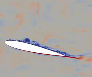
Figure 6. Snapshots of the instantaneous vorticity  $\omega _z$ contours normalised by $c$ and $U_\infty$ at $k_{red} = 0.1$. Left, smooth inflow; middle, $L_{x} = 1c$; right, $L_{x} = 1.5c$. Panels show (a) $\alpha = 15.8^\circ \uparrow$, (b) $\alpha = 21.8^\circ \uparrow$, (c) $\alpha = 23.8^\circ \uparrow$, (d) $\alpha = 24.9^\circ \uparrow$, (e) $\alpha = 18.8^\circ \downarrow$. The dashed ellipse marks the LEV's size and location as suggested in figure 7 by using the skin friction. The arrows pointing upward and downward denote airfoil pitching upstroke and downstroke, respectively.
The peak drag coefficients for large-scale inflow turbulence cases obviously decrease compared with that of the smooth inflow case (not shown). The average peak drag coefficient of the large-scale inflow turbulence cases decreased by approximately 21 % compared with that of the smooth inflow case. This apparent change in the peak drag coefficient was not observed for the small-scale FST case (e.g. Reference Kim and XieKim & Xie 2016; Reference Huang, Albers, Meysonnat, Meinke and SchröderHuang et al. 2020). This difference in the peak drag coefficient correlates well with that of the lift coefficient. It was observed that turbulence does not apparently increase the drag coefficient.
The impact of the large-scale inflow turbulence on the minimum moment coefficient is similar to that on the lift and drag coefficients. The other visible impact occurs at the dynamic stall angle and during the downstroke shown in figure 5(b). The ‘memory’ (i.e. the area in the hysteresis loop) is obviously reduced for the two large-scale inflow turbulence cases at the high angle of attack and during the downstroke, where separated flows are dominant (see the middle and right of figure 6e). Again, this is due to the impingement of the incoming large-scale turbulence, resulting in less energetic shed LEVs. This further illustrates the magnitude of the impact on the LEV structures. Overall, the free-stream large-scale turbulence clearly changes the force and moment hysteresis under the given conditions. From the data shown in figure 5, it can be concluded that the aerodynamic force coefficients are apparently changing due to the impingement of large-scale free-stream turbulence on the LEVs.
Figure 6 shows snapshots of the instantaneous spanwise component of the vorticity  $\omega _z$ at the mid-span plane at $k_{red} = 0.1$ for the smooth inflow (left), large-scale inflow turbulence cases $L_{x} = 1c$ (middle) and $L_{x} = 1.5c$ (right). In the smooth inflow case during $\alpha = 15.8^\circ \uparrow$ to $21.8^\circ \uparrow$ (left parts of figure 6a,b), the boundary layer on the suction side of the blade is largely attached, and a continuous growth of the first LEV near the leading edge is observed. For the two cases of large-scale inflow turbulence (the middle and right of figure 6a,b), boundary layer separations are visible, while the first LEVs are difficult to distinguish due to their interaction with the large-scale inflow turbulence.
In the left of figure 6(c), the first LEV has grown to maturity and is ready to detach, resulting in a significant increase in the peak lift coefficient near the dynamic stall angle  $\alpha \approx 23.3^\circ \uparrow$. This is consistent with figure 5(a). Such a phenomenon at this phase angle is not evident in the two cases of large-scale inflow turbulence cases (middle and right of figure 6c). This is because the incoming large-scale turbulence breaks down and disturbs the LEVs structures, causing the early stall and significant changes in the aerodynamic force coefficients. This is again consistent with figure 5(a,b). In addition, the pressure and skin-friction coefficients in figure 7(b–d) show further evidence of the LEVs’ suppression in the two cases of large-scale inflow turbulence.

Figure 7. Spanwise-averaged ( $0.75\le z/c \le 2.25$) surface forces at $k_{red} = 0.1$. Top, pressure coefficient; bottom, skin-friction coefficient. Panels show (a) $\alpha = 15.8^\circ \uparrow$, (b) $\alpha = 21.8^\circ \uparrow$, (c) $\alpha = 23.8^\circ \uparrow$, (d) $\alpha = 24.9^\circ \uparrow$, (e) $\alpha = 18.8^\circ \downarrow$. The arrows pointing upward and downward denote airfoil pitching upstroke and downstroke, respectively.
At  $\alpha \approx 24.9^\circ \uparrow$ near to the maximum angle of attack (left of figure 6d), the interaction between the first LEV and the first trailing edge vortex (TEV) is observed for the smooth inflow case, causing the lift to recover slightly. However, there is no evidence of the interaction between the two counter-rotating vortices in the two cases of large-scale inflow turbulence (middle and right of figure 6d), resulting in the sharp drop of the lift coefficient (see figure 5a). At $\alpha = 18.8^\circ \downarrow$ for the smooth inflow (left of figure 6e), a third LEV (second LEV not shown here) begins to form near the leading edge, resulting in a slight increase in the lift. However, for the two cases of large-scale inflow turbulence (middle and right of figure 6e), the third LEV appears very small near the leading edge, and a complete separation of the boundary layer flow is evident, mixing with the incoming large-scale turbulence. This causes a large drop in the lift coefficient within the region $15^\circ \downarrow \leq \alpha \leq 22^\circ \downarrow$ (see figure 5a).
The interaction between the large-scale inflow turbulence and the large airfoil generated eddies (e.g. LEVs) leads to breakdown, disorder and suppression during the upstroke, and disturbs the separated flows at most phase angles during the downstroke. To get a further understanding of the FST impingement on the LEVs, the surface pressure and skin-friction coefficients distributions around the pitching blade were analysed. Figure 7 shows the spanwise-averaged surface pressure and skin-friction coefficients (i.e. over  $0.75\le z/c \le 2.25$) for the smooth inflow and the two cases of large-scale inflow turbulence at the same angles of attack as those in figure 6. The values of $C_p$ (top) and $C_f$ (bottom) in figure 7(a) show the apparent emerging LEV at $x/c \approx 0.05$. However, the data from the inflow turbulence case $L_{x} = 1.5c$ suggest that a significant surface pressure variation results from the impact of the larger-scale inflow turbulence. It should be noted that the difference between the two cases of large-scale inflow turbulence (figure 7a) is simply due to the uncertainties caused by unsteadiness, as $C_p$ and $C_f$ have not been phase averaged.
The LEVs are expected to grow and convect downstream of the chord length as the pitching angle increases. Figure 7(b) shows that the centre of the LEV occurs at  $x/c \approx 0.5$, with the start at $x/c \approx 0.37$ and the end at $x/c \approx 0.7$ for the smooth inflow $C_p$ (top) and $C_f$ (bottom) at $\alpha = 21.2^\circ \uparrow$. For the two cases of large-scale inflow turbulence, the LEV extends from $x/c \approx 0$ to 0.4 at $\alpha = 21.2^\circ \uparrow$. This is consistent with figure 6(b). A similar phenomenon was observed in figure 7(c,d), which further confirms the suppression, breakdown and disordering of the LEVs due to the impact of the free-stream large-scale turbulence, which is consistent with the instantaneous vorticity contours taken at the mid-span plane shown in figure 6(c,d). The LEV average size is estimated to be 0.52 $c$ in the smooth inflow case, and 0.28 $c$ in the FST cases, indicating the significant impact of the free-stream turbulence. The decrease of the lift at $\alpha = 18.6^\circ \downarrow$ shown in figure 5(a) for the large-scale inflow turbulence cases is consistent with the $Cp$ and $C_f$ plots shown in figure 7(e). In particular, the case $L_{x} = 1.5c$ at $0.3 \leq x/c \leq 0.95$ shows a very small pressure difference between the pressure and suction sides. Moreover, the case $L_{x} = 1c$ at $\alpha = 18.6^\circ \downarrow$ shows little signature of a LEV on the blade surface, which again agrees with figure 6(e).
4.2 Effect on aerodynamic characteristics for $k_{red} = 0.2$

The effect of large-scale FST on the aerodynamic characteristics of the airfoil pitching at  $k_{red} = 0.2$ was studied (figure 8). Overall, the large-scale FST does not significantly change the lift hysteresis loop. The angle of the peak lift is almost the same as in the smooth inflow case. The large-scale FST has no apparent effect on the peak lift coefficient. The lift coefficient decrements are visible during the downstroke. The drag coefficient (not shown) decreases by an average of 15 % for the free-stream turbulence cases compared with the smooth inflow, which is of much smaller magnitude compared with $k_{red} = 0.1$ (§ 4.1). The drag coefficient in the pre-stall phase shows no visible difference between the smooth inflow and turbulent inflow cases.

Figure 8. Effect of large-scale turbulence. (a) Lift and (b) moment coefficients,  $k_{red} = 0.2$. The arrows denote the airfoil pitching direction.
The lift coefficients in the pre-stall and post-stall regimes do not change significantly for the large-scale inflow turbulence cases compared with the smooth inflow case. It was observed that, for both  $k_{red} = 0.1$ and 0.2, large-scale inflow turbulence does not consistently enhance the lift coefficients during the downstroke, which is opposite to the lift coefficient increment observed for small-scale inflow turbulence effects reported in wind tunnel tests (Reference Amandolèse and SzéchényiAmandolèse & Széchényi 2004) and LES studies (Reference Kim and XieKim & Xie 2016; Reference Huang, Albers, Meysonnat, Meinke and SchröderHuang et al. 2020). In addition, the reason for a less visible effect on the lift coefficient hysteresis loop compared with that for $k_{red} = 0.1$ could be due to the fast pitching motion, which breaks down the incoming large-scale eddies into smaller ones. Reference Kim and XieKim & Xie (2016) estimated that the convective velocity of eddies passing over the airfoil was approximately $U_{conv}=U_\infty /4$ in small-scale FST (e.g. the integral length $0.1c$), giving a dimensionless pass-through time $U_\infty /(U_{conv})=4$. The dimensionless oscillation periods for $k_{red}=0.1$ and 0.2 are 31 and 16, respectively. Considering the large-scale FST, the convective velocity is even smaller. One quarter of the oscillation period for $k_{red}= 0.2$ is shorter than the eddy pass-through time, resulting in a much more dominant role of the oscillation compared with $k_{red}= 0.1$.
The most obvious impact of FST at  $k_{red} = 0.2$ is on the moment coefficient at the stall angle and during the downstroke. Figure 8(b) shows a significant increase in the global minimum moment coefficient for the two inflow turbulence cases compared with the smooth inflow case. The peak-to-peak difference in the global minimum moment coefficient between the smooth inflow and turbulent inflow cases at is approximately 56 %. A similar effect on the moment coefficient was observed for $k_{red} = 0.1$ (figure 5b). Given that large-scale FST has a significant impact on the location of the aerodynamic force centre of the pitching blade, it can be concluded that the global minimum moment coefficient is strongly dependent on the free-stream turbulent quantities. Overall, the high-frequency pitching motion of the blade ( $k_{red}=0.2$) mitigates the impact of large-scale FST on the aerodynamics. An extensive analysis of the vorticity contours, surface pressure and skin-friction coefficients confirms this. In the following sections, only data for $k_{red}=0.1$ will be discussed.
4.3 Dispersive shear stress in the wake
To quantify the contribution of the pitching motion to momentum transfer in the wake, the term ‘dispersive stress’ is used. The dispersive stress is derived based on a ‘triple’ decomposition
 \begin{equation} {u}_{i}(t) = \langle \tilde{{u}}_{i} \rangle + \hat{u}_{i} + {u}'_{i}(t), \end{equation}
where  ${u}_{i}(t)$ is the instantaneous time velocity ( $i$ denotes $u,v,w$), $\langle \tilde {{u}}_{i} \rangle$ is the average of the entire cycle of the phase-average velocity (4.2), $\hat {u}_{i} = \tilde {{u}}_{i} - \langle \tilde {u}_{i} \rangle$ is the phase fluctuation of the phase-averaged velocity, $\tilde {{u}}_{i}$ is the phase-averaged velocity and ${u}'_{i}(t) = {u}_{i}(t) - \tilde {{u}}_{i}$ is the LES resolved instantaneous fluctuations
 \begin{equation} \langle \tilde{{u}}_{i} \rangle = \frac{1}{2\pi}\int_{0}^{2\pi} \tilde{{u}}(\psi)\,\text{d}\psi. \end{equation}
The production of phase fluctuations  $\hat {u} \hat {u}$ and $\hat {u} \hat {v}$ are the dispersive normal stress and dispersive shear stress, respectively, at the phase angle $\psi$; $\langle \hat {u} \hat {u} \rangle$ and $\langle \hat {u} \hat {v} \rangle$ are the averaged dispersive normal stress and dispersive shear stress, respectively, over the entire cycle; $\widetilde {u'u'}$ and $\widetilde {u'v'}$ are the phase-averaged turbulent normal stress and turbulent shear stress at the phase angle $\psi$, respectively.
The post-processing of the phase stress data presented in this section was obtained from time series of 75 000 time steps (three cycles) each at five wake probes whose coordinates were  $x/c = 2$, $y/c = 0$ and $z/c = 1$, 1.25, 1.5 1.75 and 2, respectively. At $x/c = -3.5$, $y/c = 0$, and $z/c = 1.25$, 1.5 and 1.75, time series of 50 000 time steps were sampled each at the three upstream probes. Considering the homogeneity in the spanwise direction in the sampled region, 6 and 15 cycles of ${u}_{i}(t)$ were phase averaged to obtain the final phase-averaged velocity $\tilde {u}_{i}$ for the upstream and the wake probes, respectively.
Figure 9 shows comparison of the phase-averaged velocity  $\tilde {{u}}_{i}$ at the upstream location ( $x/c = -3.5$, $y/c = 0$) and the wake location ( $x/c = 2$, $y/c = 0$), for the case $L_{x} = 1c$. The streamwise phase-averaged velocity $\tilde {u}$ oscillates at the upstream probes ( $x/c = -3.5$, $y/c =0$), because the pitching period is several times the integral time scale of the FST, and the averaging is effectively only 6 pitching periods. At the wake probe $x/c = 2$, the streamwise phase-averaged velocity $\tilde {{u}}$ is dominated by the slow blade pitching motion, with some high-frequency fluctuations. The velocity deficit in the wake is evident at most phase angles, with a maximum just after the maximum angle of attack at $\psi =90^\circ$. A similar trend is observed in the two cases $L_{x} = 1c$ and $L_{x} = 1.5c$ (not shown).

Figure 9. Phase-averaged velocity  $\tilde {u}_{i}/U_\infty$ at $k_{red} = 0.1$. Case $L_{x} = 1c$. Panels show (a) $x/c = -3.5$, $y/c = 0$, (b) $x/c = 2$, $y/c = 0$. See figure 1 for the phase angle $\psi$ and the angle of attack $\alpha$.
The cross-flow phase-averaged velocity  $\tilde {{v}}$ and the spanwise phase-averaged velocity $\tilde {{w}}$ are very small at the upstream probes for both cases (figure 9a). A correlation is visible between $\tilde {{u}}$, $\tilde {{v}}$ and $\tilde {{w}}$. This is again due to the short phase average at the upstream probes. The cross-flow velocity $\tilde {{v}}$ at the wake station is very sensitive to the vortex shedding, e.g. at $\psi \approx 90^\circ$ when the first LEV and the first TEV detach and shed into the wake (see figure 6c (left)), and causes a strong oscillation of $\tilde {{v}}$ at this phase angle.
Figure 10 shows the dispersive shear stress  ${\hat {u}\hat {v}}$, turbulent shear stress $\widetilde {u'v'}$ and turbulent kinetic energy $\widetilde {{TKE}}$ in the wake at $x/c = 2$ for the two cases $L_{x} = 1c$ and $L_{x} = 1.5c$. The dispersive shear stress $\hat {u}\hat {v}$, the turbulent shear stress $\widetilde {u'v'}$ and $\widetilde {{TKE}}$ show a very small magnitude at lower phase angles (i.e. $-90^\circ \uparrow \le \psi < 90^\circ \uparrow$), whereas, at high phase angles (i.e. $90 ^\circ \uparrow \leq \psi \leq 270 ^\circ \downarrow$), they show a significant change in magnitude. The $\widetilde {{TKE}}$ values are obviously larger at high phase angles compared with low phase angles. This is attributed to the pitching downstroke motion of the blade, resulting in dominant separated flows in the boundary layer and the shed vortices. Figure 10 shows that the dispersive shear stress $\hat {u}\hat {v}$ and the turbulent shear stress $\widetilde {u'v'}$ in the wake in figure 10(a,b) are of the same order of magnitude, but usually of opposite sign at high phase angles ( $90 ^\circ \uparrow \leq \varPsi \leq 270^\circ \downarrow$). This suggests that the dispersive shear stress often partially or entirely cancels the turbulent shear stress in the wake, resulting in less resistance to the boundary layer flow on the suction side and enhanced lift.

Figure 10. Dimensionless dispersive shear stress  $\hat {u}\hat {v}$, turbulent shear stress $\widetilde {u'v'}$ and turbulent kinetic energy $\widetilde {{TKE}}$ at $x/c = 2$, $y/c =0$ and $k_{red} = 0.1$. (a) Case $L_{x} = 1c$, (b) case $L_{x} = 1.5c$.
Table 3 shows the dimensionless cycle-averaged total dispersive shear stress  $\langle \hat {u} \hat {v}\rangle$, the dimensionless cycle-averaged total turbulent shear stress $\langle \widetilde {u'v'} \rangle$ and the dimensionless total shear stress ( $\tau _{a}$), which is the cycle-averaged sum of the dispersive shear stress and the turbulent shear stress. The total dispersive stress for the larger integral length scale case ( $L_x=1.5c$) is almost half of that for the smaller integral length scale case ( $L_x=1c$), suggesting that the FST with a large integral length scale mitigates the pitching motion effect. Assuming the integral length $L_x$ is the average eddy size and the eddy convection speed is approximately one third of the free-stream velocity (Reference Kim and XieKim & Xie 2016), the average convection time of the free-stream eddies passing over the blade for both cases $L_x=1c$ and $L_x=1.5c$ is one order of magnitude smaller than the pitching period for $K_{red}=0.1$, while the latter is 50 % closer to the pitching period. This perhaps explains why the latter mitigates the pitching motion effect. The magnitude of the total turbulent stress for the $L_x=1.5c$ case is slightly larger than that for the $L_x=1c$ case, possibly due to the smaller dissipation for the former. The large magnitude of the total dispersive stress in the wake region indicates the significant role of the large-scale unsteady flow.
Table 3. Cycle-averaged dispersive stress  $\langle \hat {u} \hat {v} \rangle$, turbulent shear stress ${\langle {\widetilde {{u}'{v}'}} \rangle }$ and total shear stress ( $\tau _a = \langle \hat {u} \hat {v} \rangle +{\langle {\widetilde {{u}'{v}'}} \rangle }$ at probes ( $x/c = 2$, $y/c =0$) for FST cases.

4.4 Quadrant analysis
To better understand the dispersive and turbulent shear stresses in the wake region, the widely used quadrant analysis (Reference Wallace, Eckelmann and BrodkeyWallace, Eckelmann & Brodkey 1972) is used. The quadrant analysis is a useful tool to gain more insight into the fractional contribution of each of the four categories of turbulent shear stress, as well as the dispersive stress. The four categories are as follows: Q1 ( $+{u}',+{v}'$), Q2 ( $-{u}',+{v}'$), Q3 ( $-{u}',-{v}'$) and Q4 ( $+{u}',-{u}'$), which are referred to as quadrants of the Reynolds stress plane (Reference Wallace, Eckelmann and BrodkeyWallace et al. 1972; Reference WallaceWallace 2016). The quadrant analysis for the dispersive stress is the same as for the turbulent stress, except that the phase fluctuations $\hat {u}_{i}$ are used instead of the turbulent fluctuations $u'_i$. Quadrants Q2 and Q4 refer to the gradient-like motion, i.e. the ejection and sweep quadrants, and they make the largest contributions to the turbulent shear stress, while Q1 and Q3 refer to the counter-gradient-like motion, i.e. the outward and inward interaction quadrants. Using the same time series as in § 4.3, this quadrant analysis technique is applied to the dispersive shear stress $\hat {u}\hat {v}$ and the turbulent shear stress ${u}{'}{v}{'}$ in the wake.
Figure 11(a,b) shows the quadrants of the turbulent shear stress  ${u}{'}{v}{'}$ for the two cases $L_{x} = 1c$ and $L_{x} = 1.5c$, respectively. The quadrants Q2 and Q4 of the turbulent shear stress for the two cases are obviously dominant compared with Q1 and Q3 (figure 11a). This means that the ejection and sweep events are the largest contributors to the turbulent shear stress in the wake flows, as in the steady turbulent boundary layer flow. However, the ejection events are slightly stronger than the sweep events. On the contrary, figure 12 shows that quadrants Q1 and Q3 are dominant for the dispersive shear stress $\hat {u}\hat {v}$ compared with quadrants Q2 and Q4. This means that the outward and inward events contribute most to the dispersive shear stress in the wake of a pitching wind turbine blade, as opposed to the turbulent shear stress (figure 11).

Figure 11. Quadrant analysis for the dimensionless instantaneous turbulent velocities  ${u}'$ and ${v}'$ at $x/c = 2$, $y/c =0$ and $k_{red} = 0.1$. (a) Case $L_{x} = 1c$, (b) case $L_{x} = 1.5c$.

Figure 12. Quadrant analysis for the dimensionless phase fluctuations  $\hat {u}$ and $\hat {v}$ at location $x/c = 2$, $y/c =0$ and $k_{red} = 0.1$. (a) Case $L_{x} = 1c$, (b) case $L_{x} = 1.5c$.
The cycle-averaged dispersive shear stresses  $\langle \hat {u} \hat {v} \rangle$ are estimated to be 0.0042 and 0.0023 for the cases $L_{x} = 1c$ and $L_{x} = 1.5c$, respectively. The positive dispersive shear stresses suggest a cancellation of the turbulent shear stress in the wake, resulting in an effective propulsion to the boundary layer flow on the suction side of the blade, and an enhancement of the lift. Overall, the pitching motion at $k_{red}=0.1$ significantly reduces the magnitude of the total shear stress in the wake. The FST with integral length scales much greater than the chord length mitigates this effect.
To have a clear understanding of the quadrant analysis in figures 11 and 12, the percentage contributions of each of the quadrants for the dimensionless instantaneous turbulent velocities  ${u}'$ and ${v}'$ and the dimensionless phase fluctuations $\hat {u}$ and $\hat {v}$ for the cases $L_{x}$ = 1 $c$ and $L_{x} = 1.5c$ have been given. Figure 13(a) confirms that Q2 and Q4, which are the ejection and sweep mechanisms, make dominant contributions, as was seen in the quadrant analysis in figure 11. Similarly, for the dimensionless phase fluctuations (figure 13b), Q1 and Q3, which are the inward and outward mechanisms, are the dominant quadrants and are consistent with the quadrant analysis in figure 12. This further evidences that the turbulent shear stress and dispersive shear stress in the wake have opposite mechanisms.


5. Discussions and concluding remarks
The paper reports on the LES study of the impact of large-scale FST. The impact of large-scale FST of streamwise integral length scale,  $L_{x} \geq 1c$ and $TI = 11\,\%$ on the lift, drag and moment coefficients of the pitching wind turbine blade at the reduced frequency $k_{red}=0.1$, whose pitching period is one order of magnitude greater than the eddy convection time over the airfoil, is evident. The magnitude of the lift and drag, especially the peak values, are obviously reduced by the large-scale FST. These are attributed to the early separation of the boundary layer during the upstroke and the disordered, broken down and slow convecting LEVs, which suffer from the impingement of the incoming large-scale turbulence. This is consistent with the argument that large-scale FST reduces the aerodynamic performance of static aerofoils (Reference MahmoodilariMahmoodilari 2012; Reference Herbst, Kähler and HainHerbst et al. 2018; Reference Wang and XiaoWang & Xiao 2021). It should be noted that the small-scale FST (e.g. $L_x/c\le 0.3$) (Reference Kim and XieKim & Xie 2016; Reference Huang, Albers, Meysonnat, Meinke and SchröderHuang et al. 2020) increases the lift during the downstroke and the aerodynamic performance. This suggests the crucial role of the integral length scales in the study of the FST effect.
At a higher pitching frequency (i.e.  $k_{red} = 0.2$), where the pitching period is approximately five times the eddy convection time over the airfoil, the effect of the large-scale FST on the lift coefficients is apparently mitigated, compared with a lower reduced frequency $k_{red} = 0.1$. This is because the time scale of the dominant periodic pitching motion is close to that of the incoming turbulence, resulting in an weakened impact of the FST.
The pitching motion of the wind turbine contributes significantly to the total wake shear stress. The cycle-averaged dispersive shear stress in the wake is of the same magnitude but with an opposite sign compared with the cycle-averaged turbulent shear stress. This has two important implications: (i) the dispersive shear stress often partially or completely cancels the turbulent shear stress in the wake, resulting in less resistance to the boundary layer flow on the suction side and enhanced lift and (ii) the large-scale and slow unsteady flow in the wake plays a crucial role in the extremely long-distance convection in the wake, as such a near two-dimensional large-scale flow has weak dissipation.
In summary, for the Reynolds number considered, FST with integral length scales close to or greater than the chord length can apparently reduce the lift coefficient, whereas FST with integral length scales much smaller than the chord length increases the lift coefficient, especially during the downstroke of a pitching airfoil (e.g. Reference Kim and XieKim & Xie 2016). The dispersive shear stress is demonstrated to be an effective measure to quantify the crucial contribution of the pitching-motion-scale flow to the wake momentum exchange. Nevertheless, the impact of the large-scale FST and the blade pitching motion on the wake dynamics deserves further investigation. It is to be noted that these quasi-two-dimensional large-scale flow structures have low dissipation and can be convected to an extremely long distance downstream.
Acknowledgement
The authors are grateful to the United Kingdom Turbulence Consortium (UKTC) computational resources support under grant EPSRC, for access to ARCHER high-performance computational resources. T.E.B. appreciates the provision of the IRIDIS4 computational resources at the University of Southampton.
Funding statement
Z.T.X. is grateful for the EPSRC support (EP/M022692/1) on this study. T.E.B. is grateful for the funding support by the Petroleum Technology Development Fund (PTDF) Nigeria (PTDF/1052/17/PHD/028).
Declaration of interests
The authors declare no conflict of interest.
Supplementary material
The datasets generated during and/or analysed during the current study are available from the corresponding author on reasonable request.


 Open access