


Impact Statement
Gravure printing is a high-speed and high-quality printing technique that uses mechanically engraved metal cylinders to transfer ink to a substrate. It is suitable for a wide range of applications, including packaging, magazines, wallpaper, banknotes, printed electronics and functional coatings. Gravure printing is known for its high production speed and volume. Unlike offset printing, gravure printing transfers ink directly from the cylinder to the substrate without an intermediate cylinder.
The quality of printing can be reduced due to various types of interfacial instabilities that lead to the emergence of patterns on the coated surface. The mechanisms of these instabilities are currently being investigated for Newtonian liquids. However, most real inks are non-Newtonian. In this study, the flow in thin liquid films of inks with shear-rate-dependent viscosity is analysed theoretically and the pattern in the coated layer is investigated using an industrial gravure printing machine and a gravure printing research platform. The theory allows us to predict the width of the liquid bridge between the cylinders. It is shown that this length correlates very well with the characteristic size of the pattern.
1. Introduction
The processing of structured, thin liquid films on solid surfaces, i.e. printing, is one of the fundamental concepts of industrial production and economics. This is for the simple reason that printed surfaces have a direct impact on the perception and utility value of a product by human beings. At the same time, the costs for raw materials and energy are small, because they are calculated in essentially two and not in three dimensions. Large quantities of products can be assigned with additional value in a short time. Liquid dosing and distribution on solid surfaces are mechanically simple, by hand as well as by autonomous machinery, the printing press (Reference KipphanKipphan 2000). Once in contact with the solid, adhesion forces dominate the printed film, and fix the volatile liquid on its constraining target surface.
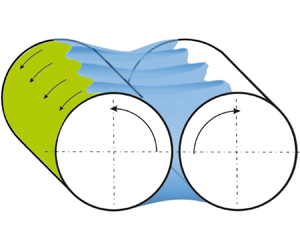
Basic configurations of liquid flow and motion of solid plates, leading to the formation of thin liquid coating films, are shown in figure 1. The configurations include lateral extraction of a plate from a liquid reservoir, lateral extraction of two parallel plates, normal retraction of two parallel plates and fluid splitting between two axiparallel rotating cylinders. In all these geometries, the solid surface is wetted with the liquid and dragged out of the reservoir with a specific velocity  $v_p$. The configuration in figure 1(d) is associated with the technology of gravure printing, considered in this paper.

Figure 1. Liquid film formation by lateral plate extraction (a), extraction of two parallel plates (b), plate retraction (c) and fluid splitting on rotating cylinders (d).
Gravure printing is a high-quality and high-speed printing method that uses metal cylinders with mechanically engraved cells to transfer ink to a substrate, which is applicable to a long list of applications (Reference Kapur, Hewson, Sleigh, Summers, Thompson and AbbottKapur et al. 2011; Reference Grau, Cen, Kang, Kitsomboonloha, Scheideler and SubramanianGrau et al. 2016; Reference Huang and ZhuHuang & Zhu 2019; Reference Tiara, Moon, Cho and LeeTiara et al. 2022). It is characterized by high production speed and volume. Industrial devices can achieve speeds of up to 15 m s $^{-1}$. This technology is suitable for long-run printing of packaging, magazines, wallpaper, banknotes and much more (Reference KipphanKipphan 2000). Other applications include printed electronics and functional coatings (Reference Grau, Cen, Kang, Kitsomboonloha, Scheideler and SubramanianGrau et al. 2016). In the gravure printing process, the ink is transferred directly from the cylinder to the substrate without an intermediate cylinder, unlike offset printing.
A very detailed theoretical and experimental study of a Newtonian flow in the liquid bridge between two rotating cylinders, associated with the gravure printing process, can be found in Reference Gaskell, Savage, Summers and ThompsonGaskell et al. (1995) and Reference Gaskell, Innes and SavageGaskell, Innes & Savage (1998). The flow field is obtained using a lubrication approximation. Then the main geometrical parameters of the liquid bridge are predicted. The predictions agree very well with the experimental data. The model includes a matching of the curvature of the flow in a thin liquid film on a cylinder with that of the meniscus of the liquid bridge between the cylinders. The problem is analogous to the Reference Levich and LandauLevich & Landau (1942) problem.
The flow is mainly determined by the capillary number  $Ca$:
$Ca$:
 \begin{equation} Ca \equiv v_p \frac{\mu}{\sigma}, \end{equation}
where  $v_p$ is the longitudinal velocity of the wall propagation, $\mu$ is the liquid viscosity and $\sigma$ is surface tension. The width $L$ of the liquid bridge, see figure 7, formed between two cylinders rotating with the same velocity $v_p$ is obtained in the form (Reference Gaskell, Savage, Summers and ThompsonGaskell et al. 1995)
 \begin{equation} L \approx 1.24 \sqrt{R h_0} Ca^{{-}1/3}, \end{equation}
where  $R$ is the cylinder radius and $h_0$ is the thickness of the coated film, determined by the total volume per unit width of the transferred ink. This model agrees very well with the experimental data for a wide range of operating parameters.
Recently, a model (Reference Dixit and HomsyDixit & Homsy 2013) for dip coating has been developed, which accounts for the elasticity of the surfaces and can also be used for a better understanding of gravure printing.
Printing allows for the consistent production of fine and detailed images with a wide density range. However, as has been pointed out by Reference KumarKumar (2015), liquid relaxation flows can give rise to instabilities under certain operating conditions, which results in spontaneous pattern formation. This is due to the presence of low-energy degrees of freedom at the highly volatile fluid meniscus at the liquid–air interface. In particular, these phenomena apply to the dynamic steady-state environment of a printing press, which keeps up a constant non-equilibrium, and provides plenty of time for an instability to grow in amplitude. Capillary levelling and waves, liquid bridge formation and interfacial and wetting instabilities determine the behaviour and the final state of the film (Reference Sauer, Roisman, Dörsam and TropeaSauer et al. 2018). Contrasting to this, phenomena like phase separation or evaporation, which depend on elevated energy scales, can be largely blanked out from understanding the process.
The fingering instability at the meniscus of a retracting liquid–air interface in a Hele-Shaw cell is very similar to the instabilities of the flows in porous media (Reference Saffman and TaylorSaffman & Taylor 1958). The linear stability of the problem (Reference Carvalho and ScrivenCarvalho & Scriven 1999) allows one to explain how the particular length scale associated with the fingering instability evolves. Important contributions have been attributed to gravure printing from gravure roll coating research. Reference Pulkrabek and MunterPulkrabek & Munter (1983) observed that the coating applied with a hashur gravure roll developed a periodic ribbing pattern with a period that was independent of the hashur period, but was essentially a function of coating layer thickness and velocity. Reverse coating, and the conditions of the ribbing instability, were studied by Reference Coyle, Macosko and ScrivenCoyle, Macosko & Scriven (1990). An effort to a principal classification of the possible flow regimes goes back to Reference Benkreira, Patel, Edwards and WilkinsonBenkreira et al. (1994). The particular influence of the gravure pattern of the cylinder has been considered by Reference Benkreira and CohuBenkreira & Cohu (1998), Reference SchwartzSchwartz (2002), Reference KapurKapur (2003), Reference Hewson, Kapur and GaskellHewson, Kapur & Gaskell (2006) and Reference Hewson, Kapur and GaskellHewson, Kapur & Gaskell (2009). Recent progress on dealing with one of the fundamental challenges of gravure printing and coating, i.e. the fact that there are interacting ink flows on very different length scales, was contributed by Reference Raske, Hewson, Kapur and de BoerRaske et al. (2017). As a matter of fact, when considering ribbing pattern length scales in printing inks, one cannot neglect the effect of ink rheology, as typical printing inks show significant shear-thinning. This has been studied by Reference Wu, Carvalho and KumarWu, Carvalho & Kumar (2018, Reference Wu, Carvalho and Kumar2019).
The coupling between fluid bulk and meniscus renders the problem a nonlinear one, even though the flow profiles can be adequately described by the linear Stokes approximation. The instability can be characterized by scaling exponents, which shift with certain system parameters, such as surface elasticity or ink rheology. The point is that the finger instability in a Hele-Shaw cell is a limiting case of that which one finds in the printing press, but that the latter is also related to other instabilities such as the Rayleigh–Taylor instability, or to even more complex mechanisms, which have not yet been fully elucidated. A recent discussion on the possible instabilities that have been observed has been presented by Reference Roisman, Abboud, Brockmann, Berner, Berger, Rothmann-Brumm, Sauer, Dörsam and HussongRoisman et al. (2023).
In this study, we characterize the pattern formation that accompanies gravure printing with industrial inks of shear-rate-dependent viscosity. The viscosity of such inks can vary by several orders of magnitude, depending on the local instantaneous shear rate. This is why the existing models developed for Newtonian liquids (Reference Gaskell, Savage, Summers and ThompsonGaskell et al. 1995, Reference Gaskell, Innes and Savage1998) cannot be directly applied. The characteristic size of the pattern, produced by instabilities that accompany gravure printing on an industrial printing machine, is measured for a wide range of operating conditions, including the thickness of the coating film and the rotational velocity of the cylinders. An optically accessible printing research platform, which is equipped with a high-speed camera, is used to visualize the temporal evolution of the instability and yields measurements of the liquid bridge width. Additionally, to better understand the development of the instabilities leading to the pattern formation, liquid bridge stretching experiments between two parallel plates are performed.
Next, a theoretical model for the liquid flow is developed, which accounts for the complex rheology of the used printing liquids. The model allows prediction of the width of the liquid bridge between the cylinders, formed during gravure printing. It is applicable to liquids of shear-rate-dependent viscosity, including yield stress liquids.
Finally, it is shown that the size of the printing pattern is of the same order as the liquid bridge width and depends on it nearly linearly.
2. Experimental method
Two different printing machines are used for the gravure printing experiments within this work: an industrial printing machine (§ 2.1) and a printing research platform (§ 2.2). The industrial printing machine serves as a tool for the creation of large-area printouts that show fingering patterns of different scales. The printouts are digitized and the distance between the fingers is measured. Since an industrial printing machine does not offer the possibility of measuring the meniscus length, we additionally use our optically accessible printing research platform. There, measurements of the meniscus length are possible from in situ high-speed video recordings of the printing nip. The engraving of the printing form as well as the printing inks used are chosen the same for both printing machines; thus the experimental results from both machines are complementary. However, there also exist some major differences between the industrial printing machine and the printing research platform. First, the nip in the industrial printing machine has a cylinder–cylinder geometry, whereas the printing research platform uses a cylinder–plate geometry. Second, the industrial printing machine is fed with a paper substrate, which is pressed onto the rigid printing cylinder by an elastic, rubber-coated impression roller (soft-on-hard set-up), whereas the printing research platform uses a rigid glass substrate, which is pressed to the rigid printing cylinder (hard-on-hard set-up).
Two different printing fluids are used for this work. The first fluid is called ink A here. It is a commercial, bluish-red, water-based gravure ink (R0001235761, Sun Chemical Group GmbH, Niedernhausen, Germany) with a delivery viscosity of around 30 seconds efflux time in a 4 mm DIN flow cup (DIN 53211). The second fluid is called ink B, which is the same bluish-red gravure ink but diluted with water to an efflux time of 14 seconds. Measurements of viscosity over the shear rate at 20  $^\circ$C are performed with a rotational rheometer (Lab+, NETZSCH-Gerätebau GmbH, Selb, Germany) for both fluids after formulation. A cone–plate geometry with a cone diameter of 60 mm and an opening angle of 1 $^\circ$ is used.
Since the shelf-life of inks A and B is limited (ink A, several months; ink B, a few weeks), we have to use different batches and reformulations of the ink for the industrial printing experiments (§ 2.1), the experiments on the printing research platform (§ 2.2) and the liquid bridge stretching experiments (§ 2.3.2). This leads to slightly different viscosities of the inks among the different experimental set-ups. Measurements of viscosity over shear rate for all fluids used can be found in figure 2. The inks for the industrial printing machine are called inks A-1 and B-1, the inks for the liquid bridge set-up are called inks A-2 and B-2 and the ink for the printing research platform is called ink B-3. Each data point in figure 2 is the mean of three measurements. The standard deviation of the three measurements is not plotted since it is around 1 % to 3 % for all data points. For this study, we only use the viscosity measurements of inks A-1 and B-1 from the industrial printing experiments (figure 2), since these experiments are the focus of this work and are used to determine the characteristic size of the printed patterns  $\ell$.

Figure 2. Viscosity  $\mu$ as a function of the shear rate $\dot \gamma$ for inks A and B, as used in the different experimental set-ups: industrial printing machine (- $1$), liquid bridge set-up (- $2$) and printing research platform (- $3$).
$3$).
The shear stresses  $\tau = \mu \dot \gamma$ for relatively small shear rates $\dot \gamma < 1$ s $^{-1}$ are shown in figure 3. Ink A-1 demonstrates the properties of a yield stress fluid. The estimated yield stress is $\tau _Y=0.61$ Pa. The yield stress for ink B-1 is smaller than $0.1$ Pa and its exact value cannot be determined by the extrapolation of the existing data. The yield shear stress for ink B-1 is neglected in the further analysis.

Figure 3. Shear stresses  $\tau$ of inks A-1 and B-1 at low shear rates $\dot \gamma <1$ s $^{-1}$. The estimated yield shear stress for ink A-1 is $\tau _Y=0.61$ Pa, obtained by extrapolation of the data to $\dot \gamma =0$.
The surface tension of all fluids used is measured using a drop shape analyser (DSA 100, Krüss, Hamburg, Germany) in pendant drop mode at temperatures between 22 and 26  $^\circ$C. Twenty droplets are measured per fluid. The results are shown in table 1.
Table 1. Surface tension  $\sigma$ of all fluids used.

2.1 Industrial gravure printing machine
Gravure printing experiments are performed on an industrial printing web-press (Gallus RCS 330-HD, Gallus Ferd. Rüesch AG, St Gallen, Switzerland). Printing velocities up to 2.667 m s $^{-1}$ with a maximum printing width of 330 mm can be achieved with the machine. For this study, experiments with two different water-based gravure printing inks (inks A-1 and B-1) at printing velocities of 0.083, 0.167, 0.25, 0.5, 1, 1.5 and 2 m s $^{-1}$ are conducted. The values in m s $^{-1}$ were converted from integer values in m min $^{-1}$, which is a common unit in the printing industry, and then rounded to three decimal places. In printing form, an electromechanically engraved, chromium-plated copper printing cylinder with a radius 72.75 mm on a steel body is employed. The engraving has a raster angle of $\alpha _r=59.35^\circ$, which corresponds to HELL engraving angle no. 2, and four different raster frequencies $f_r=[60, 70, 80, 100]$ lines cm $^{-1}$. The engraved cells are pyramid-shaped and have an opening angle of 120 $^{\circ }$, which equals the diamond stylus angle used for engraving.
The thickness of the printed film  $h_0$ strongly depends on the volume of the engraved cells on the printing cylinder per area, the so-called dip volume $V_{{dip}}$. First, the mean volume $\bar {V}$ of the engraved cells on the printing cylinder used in the industrial experiments is measured using a three-dimensional optical profilometer (PLu neox, Sensofar DACH, Langen, Germany) in confocal mode. For each of the four raster frequencies $f_r=[60, 70, 80, 100]$ lines cm $^{-1}$, three cells are measured and the average is used as the mean volume $\bar {V}$. The three-dimensional surface data are analysed in MATLAB 2022b, using the algorithm from Reference SchäferSchäfer (2019). Second, the dip volume $V_{{dip}}$ is calculated using (Reference SchäferSchäfer 2020)
 \begin{equation} V_{{dip}} = \frac{\bar{V} {f_r}^2}{\sin2\alpha_r}, \end{equation}
where  $V_{{dip}}$ is the dip volume, $\bar {V}$ is the mean volume of three cells, $f_r$ is the raster frequency and $\alpha _r$ is the raster angle.
To estimate the thickness of the (wet) printed film  $h_0$, we use
 \begin{equation} h_0\approx0.5 V_{{dip}}. \end{equation}
 We emphasize that this is just a rough approximation of  $h_0$, since $h_0$ depends on the transfer volume. The transfer volume also is a fraction of $V_{{dip}}$, but it is dependent on ${Ca}$ (see Reference Grau, Cen, Kang, Kitsomboonloha, Scheideler and SubramanianGrau et al. 2016). All determined values for $h_0$ are shown in table 2.
Table 2. Thicknesses of the printed film  $h_0$, estimated with (2.2).

Since the focus of this study is fingering instabilities, printed patches of size  $64\,{\rm mm}\times 180\,{\rm mm}$ with a tonal value of 100 % are used. This tonal value is equivalent to the highest possible transfer volume. At high transfer volumes, a continuous meniscus is formed in the printing nip, and the ink splitting regime of lamella splitting is observed, which accompanies fingering instabilities. These instabilities lead to finger patterns on the printed substrate. In contrast, at lower tonal values, we observe the regime of point splitting, which leads to dot patterns on the substrate. The printed dot patterns correspond to the engraved raster pattern on the printing cylinder (Reference Brumm, Weber, Sauer and DörsamBrumm et al. 2021, Reference Brumm, Ciotta, Sauer, Blaeser and Dörsam2023).
A sketch of the gravure unit of the industrial printing machine is shown in figure 4. The engraved cells on the printing cylinder (1) are filled with ink from the doctor blade chamber (4). The excess ink is wiped away by the doctor blade (with a doctor blade angle of  $-37^\circ$), which leaves only a thin lubrication film on the walls between the cells. The substrate (6), onto which the ink is deposited, first passes a deflector roll (3) and is then guided through the nip between the printing cylinder and pressure roller (2). The pressure roller applies a high pressure onto the substrate so that the ink from the cells is transferred to the substrate. In this work, we use a coated paper substrate (Sigmakraft RTC Green, Mosaico Specialty Papers, Altavilla Vicentina, Italy) with a grammage of $70\,{\rm g}\,{\rm m}^{-2}$. The printed layer of ink is subsequently dried in a hot air and infrared dryer (5).

Figure 4. Sketch of the gravure printing unit within the industrial printing machine Gallus RCS 330-HD. (1) Printing cylinder, (2) pressure roller, (3) deflector roller, (4) doctor blade chamber filled with printing ink, (5) hot air and infrared drying unit, (6) substrate.
The printed substrate is digitized using a colour-calibrated flatbed scanner (Epson Perfection V850 Pro, Seiko Epson Corporation, Suwa, Japan) at high resolution of 2400 dpi ( $10.58\,\mathrm {\mu }$m px $^{-1}$). The scans reveal spontaneous finger pattern formation phenomena created during fluid transfer in the printing nip. The distance $\ell$ between the fingers is determined with the method from Reference Brumm, Sauer and DörsamBrumm, Sauer & Dörsam (2019), which uses one-dimensional fast Fourier transform perpendicular to the printing direction and subsequent peak-finding within the averaged frequency spectrum. The algorithm is implemented in MATLAB 2022b using the fft function. For both printing fluids (inks A-1 and B-1), experiments with 28 parameter combinations of raster frequency $f_r$ and printing velocity $v_p$ are conducted. For each parameter combination, eight printed patches are analysed.
2.2 Gravure printing research platform
The gravure printing research platform is the second experimental set-up used for gravure printing experiments within this work. It complements the industrial gravure printing machine since it offers optical accessibility to the printing nip and in situ observation of the meniscus shape. Measurements of the meniscus length are possible as well. The development of our research platform is inspired by the experimental set-up of Reference Schäfer, Roisman, Sauer and DörsamSchäfer et al. (2019) and Reference SchäferSchäfer (2020).
A sketch of the gravure printing research platform in front view is shown in figure 5 and a side view in figure 6. The engraved cells of the gravure printing cylinder with a radius 110 mm (1) are filled using a doctor blade (9), onto which printing fluid has been pipetted. The key component of the research platform is the custom-built, optically accessible substrate carrier (4), onto which a Gorilla glass substrate (Corning Incorporated, Corning, NY, USA) of size  $207\,{\rm mm}\times 90\,{\rm mm}\times 1.1\,{\rm mm}$ is mounted (5). Inside the substrate carrier, there is a gold-plated prism (7), which reflects the white light from a high-power, cold-light light-emitting diode (LED) (LED8, StarLight Opto-Electronics GmbH and Co. KG, Nuremberg, Germany) (3). In the set-up, a $\times \,12$ zoom objective (Navitar, Rochester, NY, USA) (8) with coaxial illumination and aperture is used in combination with a high-speed camera (Fastcam Nova S12, Photron Deutschland GmbH, Reutlingen, Germany) (6). The optically accessible substrate carrier is pressed onto the printing cylinder with a pressure roller while it passes the nip with the printing velocity $v_p$. Printing pressures between 2 and 16 N mm $^{-1}$ and printing velocities between 0.1 and 3 m s $^{-1}$ can be realized.

Figure 5. Sketch of the gravure printing research platform in front view. (1) Printing cylinder, (2) impression roller, (3) high-power LED, (4) optically accessible substrate carrier, (5) glass substrate (light blue), (6) high-speed camera, (7) gold-plated prism (orange), (8) Navitar zoom objective, (9) doctor blade.

Figure 6. Sketch of the gravure printing research platform in side view. (1) Printing cylinder, (2) impression roller, (3) high-power LED, (4) optically accessible substrate carrier, (5) glass substrate (light blue), (6) high-speed camera, (7) gold-plated prism (orange), (8) Navitar zoom objective.
The high-speed camera is operated with a frame rate of 30 000 fps, an aperture time of 1/60 000 s and a resolution of  $640\,{\rm px}\times 480\,{\rm px}$. Thus, a field of view of around $22\,{\rm mm}\times 16\,{\rm mm}$ with a spatial resolution of $34\,\mathrm {\mu }$m px $^{-1}$ is obtained. As printing fluid, ink B-3 is used. Printing velocities of 0.25, 0.5, 1 and 2 m s $^{-1}$ are used at a printing pressure of 2 N m $^{-1}$ and a doctor blade pressure of 0.3 N mm $^{-1}$. The doctor blade angle is 64 $^{\circ }$. For the research platform, the same engraving as in the industrial printing experiments is applied to the printing cylinder (electromechanical engraving, HELL engraving angle no. 2, stylus angle 120 $^{\circ }$). Printing experiments are performed on patches of the printing cylinder, which are engraved with a raster frequency $f_r$ of 60, 80 and 100 lines cm $^{-1}$ and a tonal value of 100 %. For this study, only the meniscus length $L$ is of interest, although it would also be possible to determine the distance $\ell$ between the fingers from the high-speed videos.
2.3 Observations of instabilities during printing
2.3.1 Pattern of instabilities observed after gravure printing
The flow configuration associated with the gravure printing is shown schematically in figure 7. The flow includes a liquid bridge formed between two rotating cylinders. The width of the liquid bridge  $L$ is determined by the total volumetric flux of the ink, by tangential speed $v_p$ of rotation of the cylinders and by the ink's rheological and interfacial properties. The main geometrical and kinematic parameters determining the problem are defined in figure 7(a). The shape of the meniscus is influenced by the appearance of the interfacial instabilities. These instabilities are shown schematically in figure 7(b). The thin deposited liquid films on the cylinders are not shown in figure 7(b) for better clarity.

Figure 7. Flow configuration associated with gravure printing. Sketch of the rotating cylinders, liquid bridge of ink and formation of a coating film. (a) Close-up sketch showing variables. (b) Three-dimensional sketch showing fingering at the meniscus between rolls.
A set of high-speed video images of the flow in the liquid bridge at various operational conditions are shown in figure 8. The images in figure 8 also show the emergence of geometric finger patterns on the printed surfaces. A zoomed-in image of the region of interest can be found in figure 9.

Figure 8. Exemplary high-speed video frames recorded with the printing research platform. Time evolves from top to bottom, as indicated by the time stamps. The printing velocities  $v_p$ and raster frequencies $f_r$ are: (a) $v_p=0.25$ m s $^{-1}$, $f_r=100$ lines cm $^{-1}$; (b) $v_p=2$ m s $^{-1}$, $f_r=60$ lines cm $^{-1}$. The region of interest is indicated in each frame with a yellow rectangle, which moves from right to left with $v_p$. The region of interest shows finger patterns, which are clearly visible in (a) and smaller, with less contrast and more blurred in (b). The printing nip between the gravure cylinder and substrate is marked as a white line.

Figure 9. High-speed video frames cropped to the region of interest. (a) Zoomed-in frame from figure 8(a) at time 53 ms. The image shows the meniscus width  $L$, which is the distance between the nip and unstable meniscus on the left side of the nip. The meniscus at the right side of the nip is stable. Printing direction from left to right. (b) High-speed recording without printing fluid with $v_p=0.25$ m s $^{-1}$ and $f_r=100$ lines cm $^{-1}$. It is used to determine the position of the nip, which shows characteristic light refraction at the contact area between the glass substrate and the printing cylinder (see arrow).
The location of the nip is determined using extra-high-speed videos without printing fluid. There, the nip can be located due to light refraction at the contact region of the glass substrate and gravure cylinder.
One example of a typical scan of a printed sample from the industrial gravure printing machine is shown in figure 10. The zoomed-in images show the appearance of fingering patterns, which are oriented roughly along the printing direction. The pattern depends on the raster frequency  $f_r$, which determines also the volumetric flux of the ink.

Figure 10. Exemplary scans of a printed sample from the industrial gravure printing machine, printed with ink B-1 at  $v_p=0.083$ m s $^{-1}$. Printing direction from right to left. The scan shows four full-tone patches of size $64\,{\rm mm}\times 180\,{\rm mm}$ with different raster frequencies $f_r$: (a) 100 lines cm $^{-1}$, (b) 80 lines cm $^{-1}$, (c) 70 lines cm $^{-1}$ and (d) 60 lines cm $^{-1}$. Zoomed-in images of the fingering patterns are shown on the right. The lower the raster frequency $f_r$, the larger the distance between the fingers $\ell$.
The appearance of the finger patterns is also strongly influenced by printing velocity and choice of printing ink (see figure 11). The higher the printing velocity, the lower is the distance between the fingers and the pattern appears more blurred. In comparison with ink A-1, ink B-1 produces finger patterns with a larger finger distance. This is attributed to the lower viscosity of ink B-1.

Figure 11. Exemplary finger patterns from the industrial gravure printing machine, printed with different combinations of printing velocity and printing ink: (a)  $v_p=0.083$ m s $^{-1}$, ink A-1, (b) $v_p=2$ m s $^{-1}$, ink A-1, (c) $v_p=0.083$ m s $^{-1}$, ink B-1 and (d) $v_p=2$ m s $^{-1}$, ink B-1. The raster frequency is always $f_r=100$ lines cm $^{-1}$. The printing direction goes from right to left.
2.3.2 Finger formation during fast liquid bridge stretching
The main focus of this paper is the study of finger formation during gravure printing. However, this technology does not always allow direct observation of the formation and development of the instabilities leading to the formation of finger-like structures on the printed surfaces. This problem becomes even more challenging since the rheology of the inks is non-Newtonian since the viscosity depends on the strain rate.
The development of the fingering instability can be best observed in experiments with a much simpler geometry and well-investigated flows in a so-called lifting of a Hele-Shaw cell. This configuration is shown schematically in figure 1(c). A liquid volume in a thin initial gap between two parallel solid plates is stretched since one of the plates starts to move with a constant acceleration. The flow of the liquid in the gap is observed using a high-speed video system through a fixed transparent plate. The details of the experimental set-up and the description of the fingering instability for Newtonian liquids can be found in the literature (Reference Brulin, Roisman and TropeaBrulin, Roisman & Tropea 2020).
Two inks, ink A-2 and ink B-2, have been used in this study for the liquid bridge stretching experiments. The dependence of the ink viscosity on the shear rate is shown in figure 2.
Exemplary results of the bridge stretching are shown in figure 12, which are generated with the top-view camera. In all the considered cases, the stretching leads to the instability of the liquid interface and subsequent fingering. Several typical sizes characterize the final observed pattern of instabilities. One is the smallest distance  $\ell ^*$ between the fingers near the initial bridge edge. The second size is the typical finger length. While the finger length $L^*$ is of the same order as the initial bridge radius $R_0$, the distance between the fingers is determined by the length of the most unstable mode associated with the interfacial instability.

Figure 12. Liquid bridge stretching between two parallel plates. Examples of fingering after stretching of industrial inks used for gravure printing. The initial gap thickness  $H_0$ is in the range from 40 to 55 $\mathrm {\mu }$m in all presented experiments. The plate acceleration and the liquid are (a) $a=5$ m s $^{-2}$, ink A-2, (b) $a=10$ m s $^{-2}$, ink A-2, (c) $a=5$ m s $^{-2}$, ink B-2 and (d) $a=10$ m s $^{-2}$, ink B-2, respectively.
The mechanisms leading to the appearance of the interfacial instabilities, relevant to this study, are often explained by the balance of the forces associated with the positive pressure gradient at the interface and capillary forces. This includes the well-known Rayleigh–Taylor instability, driven by the pressure gradient caused by gravity or acceleration, and Saffman–Taylor instabilities (Reference Saffman and TaylorSaffman & Taylor 1958) in which the pressure gradient at the interface is the result of the liquid flow through a porous media. The same mechanism leads also to the emergence of fingers in a liquid bridge formed between two plates, separating with a constant acceleration (Reference Roisman, Abboud, Brockmann, Berner, Berger, Rothmann-Brumm, Sauer, Dörsam and HussongRoisman et al. 2023). The typical distance  $l_{fingers}$ between the fingers is scaled well as
 \begin{equation} l_{fingers} \sim \sqrt{\frac{\sigma}{p_{,n}}}, \end{equation}
where the pressure gradient in the axisymmetric case is  $p_{,n}=\partial p/\partial r$. This scaling agrees well with numerous experimental data (Reference Brulin, Roisman and TropeaBrulin et al. 2020), including the data from this study, shown in figure 12. However, the theoretically predicted distance $l_{fingers}$ is two orders smaller than the observed distance of the fingers on the printed samples, as shown in figure 11. Therefore, some additional physical factors play a role in the formation of these fingers. This is the topic of further analysis.
3. Flow of an ink of shear-rate-dependent viscosity
In this section, a flow of ink is considered in two main regions. First, the ‘inner solution’ in the thin coating flow is analysed accounting for the viscosity dependence on the local shear rate. Next, the inner solution is matched with the outer solution in the liquid bridge between two cylinders. The solution allows estimation of the width of the liquid bridge under various operating conditions.
Consider a steady liquid flow in a liquid bridge between two symmetric cylinders of radius  $R$ rotating with the same angular velocity $\omega$. The sketch of the flow in the bridge is shown in figure 7.
The smallest distance between the cylinders at the symmetry plane is denoted  $2 h_0$. The distance $d$ between the cylinders is determined by the transverse $z$ coordinate. For small distances from the cylinders’ symmetry plane the expression for $d$ can be linearized, which yields
 \begin{equation} d = 2 h_0 + \frac{z^2}{R}. \end{equation}
 The distance of the liquid bridge meniscus to the axis plane is denoted  $L$. The motion of the cylinders leads to their wetting by the printing liquid. The flow in the coating liquid film is similar to the well-known dip coating problem (Reference Levich and LandauLevich & Landau 1942). This flow is considered in the following section, accounting for the complex rheology of industrial printing liquids.
3.1 Thin-film flow
Consider a steady flow in a thin liquid film of ink, extruded from a steady meniscus by a rotating cylinder, as shown in figure 7(a). Denote a lateral coordinate  $x$ along the film and the normal coordinate $y$. The origin of the coordinate system is fixed at the free film interface. The system is curvilinear. However, since the film thickness $h(x)$ is much smaller than the cylinder radius $R_0$, the curvature effects are neglected in this theory. The considered problem is steady; therefore the total volumetric flux $Q$ per unit film width
 \begin{equation} Q = h_0 v_p \end{equation}
is constant in each film cross-section:
 \begin{equation} \int_0^h u(y)\,\mathrm{d}y = Q, \end{equation}
where  $h_0$ is the asymptotic value for the film thickness far from the meniscus.
The long-wave approximation of the momentum balance equation yields
 \begin{equation} p_{,x}(x) = \frac{\partial \tau(\dot\gamma)}{\partial y},\quad \dot\gamma = u_{,y},\quad \tau(\dot\gamma) = \mu(\dot\gamma) \dot\gamma, \end{equation}
where the viscosity  $\mu (\dot \gamma )$ and the shear stress $\tau (\dot \gamma )$ are functions of the shear rate $\dot \gamma$, which can be determined for a specific liquid. This approximation is based on the assumption, typical for the analysis of thin films, that the velocity gradients in the $y$ directions are much larger than the velocity gradients in the $x$ directions. The latter thus can be neglected.
The no-slip boundary conditions at the wall  $y=h$ and the zero-shear-stress conditions at the free film interface $y=0$ yield
 $$\begin{gather} u = v_p \quad \mathrm{at}\ y = h, \end{gather}$$
 $$\begin{gather}\dot\gamma = 0 \quad \mathrm{and} \quad u = u_0\quad \mathrm{at}\ y = 0, \end{gather}$$
where  $u_0$ is an unknown velocity at the film free interface.
Note also that the momentum of the flow in the  $y$ direction, normal to the wall, is negligibly small. Therefore, also the pressure gradient $p_{,y}$ can be neglected. The pressure $p$ is, therefore, a function only of the $x$ coordinate, and is uniform along the film cross-section:
 \begin{equation} p_{,y} = 0. \end{equation}
The solution of (3.4a–c) for the velocity field is obtained with the help of the conditions (3.5)–(3.7) in the form
 $$\begin{gather} y(\dot\gamma) = \frac{\tau(\dot\gamma)}{p_{,x}}, \end{gather}$$
 $$\begin{gather}u(\dot\gamma) = u_0 + \frac{1 }{p_{,x}} \int_0^{\tau}{\dot\gamma}\,{\rm d}\tau. \end{gather}$$
 We note that the shear rate  ${\dot \gamma }$ is not constant across the liquid film, but is a function of $y$ and the still unknown velocity $u_{0}$ of the film interface. The dissipation density function $f(\dot \gamma ) = \int _0^{\tau }{\dot \gamma }\,{\rm d}\tau$, which appears on the right-hand side of (3.9), and the shear stress $\tau (\dot \gamma )$ encode the particular liquid rheological properties of the film as a function of the shear rate $\dot \gamma$:
 $$\begin{gather} \tau(\dot\gamma)\equiv\dot\gamma\mu(\dot \gamma), \end{gather}$$
 $$\begin{gather}f(\dot\gamma)\equiv \int_0^{\tau}{\dot\gamma}\,{\rm d}\tau = \dot\gamma \tau(\dot\gamma)-\int_0^{\dot\gamma}\tau(\xi)\,\mathrm{d}\xi, \end{gather}$$
where  $\xi$ is a dummy variable for integration.
Denote by  $\dot \varGamma$ the limiting value of the shear rate $\dot \gamma$ at the wall $y=h$. Equations (3.8) and (3.9) can be written for the point $y=h$ with the help of the boundary conditions (3.5)–(3.6a,b) in the following form:
 $$\begin{gather} h = \frac{ \tau(\dot \varGamma)}{ p_{,x}}, \end{gather}$$
 $$\begin{gather}u_0 = v_p- h\dot\varGamma + h\frac{\displaystyle\int_0^{\dot\varGamma}\tau(\xi)\,\mathrm{d}\xi}{\tau(\dot \varGamma)}. \end{gather}$$
 Next, the definition (3.3) of the flux in the liquid film allows writing the expression for  $Q$ in terms of $\dot \gamma$ and the interface shear rate ${\dot \varGamma }$:
 \begin{equation} Q = \frac{1}{ p_{,x}} \int_0^{\dot\varGamma} u(\dot\gamma)\tau'(\dot\gamma)\,\mathrm{d}\dot\gamma. \end{equation}
Substituting (3.9) and (3.12) in expression (3.14) yields
 \begin{equation} Q = u_0 h + \frac{h^2}{\tau^2(\dot\varGamma)} \int_0^{\dot\varGamma} f(\dot\gamma)\tau'(\dot\gamma)\,\mathrm{d}\dot\gamma. \end{equation}
Let us introduce for simplicity a function
 \begin{equation} \varOmega(\dot\varGamma) = \frac{h v_p-Q}{h^2}. \end{equation}
This function can also be expressed in terms of  $\dot \varGamma$ and the rheological properties of the liquid. The expression is obtained by accounting for expressions (3.13) and (3.15) in (3.16):
 \begin{equation} \varOmega(\dot\gamma) = \dot\gamma- \frac{\displaystyle\int_0^{\dot\gamma}\tau(\xi)\,\mathrm{d}\xi}{\tau(\dot\gamma)}- \frac{\displaystyle\int_0^{\dot\gamma}f(\xi)\tau'(\xi)\,\mathrm{d}\xi}{\tau^2(\dot\gamma)}. \end{equation}
 Function  $\varOmega$ allows us to determine the values of $\dot \varGamma$ and the corresponding wall shear stress $\tau (\dot \varGamma )$ for a given volumetric flux:
 \begin{equation} \dot\varGamma = \varOmega^{{-}1} \left( \frac{h v_p-Q}{h^2} \right),\quad \tau(\dot\varGamma) = \tau\left[\varOmega^{{-}1} \left( \frac{h v_p-Q}{h^2} \right)\right], \end{equation}
where  $\varOmega ^{-1}(\cdot )$ is an inverse function of $\varOmega (\cdot )$. In figure 13 the function $\tau [\varOmega ^{-1}(\xi )]$, computed using (3.18a,b) and the rheological properties of the corresponding liquid, is shown as a function of a dummy variable for integration $\xi$ for both inks used for the gravure printing experiments.

Figure 13. Function  $\tau [\varOmega ^{-1}(\xi )]$ computed for inks A-1 and B-1. This function is used in the expression for the wall stress (3.18a,b) with $\xi = (h v_p - Q)/h^2$.
Next, the long-wave approximation of the Young–Laplace equation, valid for the case  $h_{,x}\ll 1$, can be written in the form $p = - \sigma h_{,xx}$, where $\sigma$ is surface tension. The evolution equation for the film thickness $h(x)$ is thus obtained by substitution of this relation in (3.12), and accounting for (3.18a,b):
 \begin{equation} {\sigma} h_{,xxx} + \frac{1}{h} \tau\left[\varOmega^{{-}1}\left(\frac{h v_p-Q}{h^2}\right) \right] = 0. \end{equation}
 The argument  $v_p(h-h_0)/h^2$ on the right-hand side of (3.19) has the maximum
 \begin{equation} v_p \frac{h -h_0}{h^2} = \frac{v_p}{4h_0},\quad \mathrm{at}\ h = 2 h_0. \end{equation}
 Therefore, a characteristic shear stress  $\tau ^\star$ can be determined for a certain liquid rheology:
 \begin{equation} \tau^\star(h_0, v_p) = \tau\left[\varOmega^{{-}1}\left(\frac{v_p}{4h_0}\right) \right]. \end{equation}
 Figure 14 shows the characteristic shear stress  $\tau ^\star$ in the film flow, computed for ink B-1 for different cylinder velocities $v_p$.

Figure 14. Characteristic shear stress  $\tau ^\star$ in the film flow, defined in (3.21), computed for ink B-1 for different cylinder velocities $v_p$.
Moreover, (3.19) allows the definition of a characteristic length scale  $\lambda$ along the $x$ axis:
 \begin{equation} \lambda = \left[\frac{\sigma h_0^2}{\tau^\star}\right]^{1/3}. \end{equation}
Now, the governing equation for the evolution of the film thickness can be written in the dimensionless form
 \begin{equation} H(X) H_{,XXX}(X) - T\left[ \frac{(H -1)}{ H^2} \frac{v_p}{h_0}\right] = 0, \end{equation}
where the dimensionless variables and functions are defined as
 $$\begin{gather} h = H(X) h_0,\quad x = {-} X \lambda, \end{gather}$$
 $$\begin{gather}\tau\left[\varOmega^{{-}1}\left(\xi\right) \right] = T(\xi) \tau^\star. \end{gather}$$
Note that the sign of  $X$ is changed relative to $x$ to simplify computations.
The ordinary differential equation (3.23) can be integrated numerically for known values of  $Q$,
$Q$,  $v_p$, and the rheology of the liquids.
At high positive values of  $X$ and $H$, associated with the meniscus flow of the liquid bridge, the value of the second derivative $H_{,XX}$ asymptotically approaches a constant value denoted $K$, which is the dimensionless curvature of the meniscus. The value of the curvature is therefore
 \begin{equation} \kappa = K \frac{h_0}{\lambda^2}. \end{equation}
 The value of  $K$ depends on $\tau ^\star$ and the ratio $v_p/h_0$. For the liquids used in this study, the computed value of $K$ only very weakly depends on $v_p/h_0$. This value is $K\in [1.667\unicode{x2013}1.67]$ for ink B-1 and is $K\in [1.6\unicode{x2013}1.66]$ for ink A-1 if $10^4< v_p/h_0<10^7$. In further analysis, a constant average value $K=1.67$ is taken without significant precision loss.
3.1.1 Limiting case of Newtonian liquids
It can be shown that for a Newtonian liquid with constant viscosity  $\mu = \mu _{\mathrm {N}}$, the expression (3.17) for $\varOmega$ can be reduced to $\varOmega _\mathrm {N}(\dot \gamma )=\dot \gamma /3$. This expression with the help of (3.16) allows the derivation of the expression for the wall shear rate in a film of Newtonian liquid:
 \begin{equation} \dot\varGamma = 3 \frac{h v_p-Q}{h^2}\quad \mathrm{if}\ \mu_{{N}} = \mathrm{constant}. \end{equation}
 Taking into account that  $\tau = \mu _{N} \dot \varGamma$, the expression (3.19) is reduced with the help of (3.27) to the well-known evolution equation (Reference Levich and LandauLevich & Landau 1942):
 \begin{equation} {\sigma} h_{,xxx} + 3 \mu_{{N}}\frac{h v_p-Q}{h^3} = 0,\quad \mathrm{if}\ \mu_{{N}} = \mathrm{constant}. \end{equation}
This equation is not used in further analysis since the liquids used in the experimental part of the study are non-Newtonian. The limiting case of Newtonian liquid is considered here only to confirm the validity of the more general equation (3.19) and to make sure that no term is lost in complicated algebraic manipulations in this section.
3.2 Meniscus region of the liquid bridge and instabilities of coating
The curvature of the liquid film determines the position  $L$ of the meniscus of the liquid bridge. This distance is defined in figure 7.
For given liquid properties, thickness  $h_0$ and velocity $v_p$, the distance $L$ could be estimated from (3.1), taking into account that from geometrical considerations $d\approx 2/\kappa + 2 h_0$. Using expressions (3.1) and (3.26) yields
 \begin{equation} L = \left[\frac{\sigma h_0^2}{\tau^\star}\right]^{1/3} \sqrt{\frac{2 R}{K h_0}}. \end{equation}
 Expression (3.29) has been obtained using an assumption that the curvature of the meniscus is constant for a certain case. The same assumption was made in the theoretical study of Reference Gaskell, Savage, Summers and ThompsonGaskell et al. (1995) which allows successful prediction of the length  $L$ for Newtonian liquids. This assumption is valid only if the pressure gradient at the meniscus is not high enough to distort the meniscus shape. The pressure gradient in a viscous flow can be roughly estimated as $p_{,z}\sim \mu v_p / d^2$, where $d$ is the gap width. Therefore, the corresponding capillary length $\varDelta _c$ in the meniscus can be defined as
 \begin{equation} \varDelta_c =
\sqrt{\frac{\sigma}{p_{,z}}} = d \sqrt{\frac{\sigma}{\mu
v_p}}. \end{equation}
\begin{equation} \varDelta_c =
\sqrt{\frac{\sigma}{p_{,z}}} = d \sqrt{\frac{\sigma}{\mu
v_p}}. \end{equation}
The meniscus distortion from a cylindrical shape will be small if the ratio  $d/\varDelta _c = Ca^{1/2}$ is small. Here $Ca$ is the capillary number defined in (1.1). The observed length of the meniscus is approximately $L\approx 2$ mm. Therefore the width $d$, estimated from the geometrical considerations for the cylinder radius $R\approx 73$ mm, is $55\,\mathrm {\mu }$m. The typical shear rate in the liquid bridge for $v_p = 2$ m s $^{-1}$ is therefore $\dot \gamma \sim v_p/d\sim 10^{3}$ s $^{-1}$. The liquid viscosity at these shear rates is $\mu \sim 10^{-2}$ Pa s. Now, the capillary number calculated for these values from (1.1) is $Ca \approx 0.3$. This is why the assumption of constant curvature is valid in our range of experimental parameters.
In this study, the value of  $L$ was estimated on the printing research platform. The values were determined from selected high-speed observations, as shown in figure 9. Unfortunately, the determination of the positions of the finger pattern tips on the cylinders corresponding to $x=0$ was not feasible with truly satisfactory precision. Therefore, in this study, we confined ourselves to only tentative estimation of the values of $L$, and was measured for various velocities $v_p$ and different raster frequencies $f_r$. In figure 15, the measured values of $L$ are compared with the theoretical predictions (3.29). The theory predicts very well the order of values for $L$, and explains the dependence of $L$ on the cylinder velocity $v_p$ and the film thickness $h_0$. As mentioned above, some discrepancies can be attributed to the relatively limited precision of the measurements. Moreover, the theory does not account for the inertial effects and viscous stresses in the shearing liquid bridge between the cylinders. By this effect, the shape of the meniscus could have been deformed, and thus shifted the true value of $L$. Nevertheless, the model takes into account the major physical influencing factors.

Figure 15. Meniscus length  $L$ over printing velocity $v_p$. The measured values for $L$ come from selected high-speed observations of experiments with ink B-3 on the printing research platform. Theoretic values of $L$ are computed using (3.29).
Next, one can assume that the mechanisms of pattern formation in gravure printing are similar to the fingering instabilities observed as a result of the liquid bridge stretching, as shown in figure 12. In all the considered cases, the characteristic length of the observed tree network is comparable with the initial bridge radius  $R_0$. Following this assumption, the characteristic size $\ell$ of the printed pattern should be comparable with the liquid bridge width $L$ for gravure printing. In figure 16 the measured values of $\ell$ are shown as a function of the theoretically predicted $L$ for the range of the thicknesses $h_0\in [3.5\unicode{x2013}7.4]\,\mathrm {\mu }$m and cylinder velocities $v_p\in [0.083\unicode{x2013}2]$ m s $^{-1}$. Each data point is based on eight measurements of $\ell$ and the standard deviation of the measurements is around 1 % to 3 %, as indicated by the error bars. In all the considered cases, for both studied liquids, the ratio $\ell /L$ is between 0.35 and 0.8. Moreover, the values of $\ell$ clearly almost linearly correlate with $L$:
$L$:
 \begin{equation} \ell \approx \beta L. \end{equation}
Figure 16. Dependence of the measured characteristic size of the printed pattern  $\ell$ on the theoretically predicted width $L$ of the liquid bridge, determined by (3.29). Each data point is based on eight measurements of $\ell$. The error bars indicate the standard deviation of the measurements. The linear fit A-1 is $\ell = 0.22+0.24 L$ and the linear fit B-1 is $\ell = 0.17+0.44 L$.
The linear fit for ink A-1 yields  $\beta = 0.24$ and the linear fit for ink B-1 yields $\beta = 0.44$ (see figure 16).
The observed distance  $\ell$ between the fingers observed during the printing process cannot be modelled using the approaches based on the Saffman–Taylor-like instability. However, it correlates very well with the theoretically predicted meniscus length $L$. Moreover, the values are of the same order for all our experiments. Therefore, the appearance of the fingers in the printing samples is probably associated with the meniscus oscillations in the direction $z$, defined in figure 7. This is why the values of $\ell$ are limited by $L$.
$L$.
4. Conclusions
This experimental study shows that the mechanisms of pattern formation resulting from the liquid bridge stretching between two parallel plates and from gravure printing can be understood as similar physical concepts. In both cases, the pattern consists of tree networks of finger-like instabilities of the printed surface.
To analyse the flow associated with gravure printing, we analysed the meniscus in the printing nip of a gravure press and the patterns forming there. There are two characteristic length scales: the distance  $L$ of the meniscus from the centre of the printing nip and the finger distance $\ell$ of the viscous finger pattern, both being direct functions of printing velocity, transfer volume of the gravure pattern and the rheology of the printing inks. The dependency of finger distance on these printing parameters has been established with high precision using large-scale industrial presses, whereas the meniscus distance $L$ was studied on a laboratory press where direct optical access to the nip was possible. We developed a theoretical model for a coating flow in a thin film of non-Newtonian liquid. The model is based on the lubrication approximation. It takes into account both capillary effects and the shear-rate-dependent viscosity of the liquid. The evolution equation for a steady flow in the film is obtained, which satisfies the mass and momentum balance equations. The theory can predict the width $L$ of the liquid bridge between the rotating cylinders for the complete set of considered printing parameters. It is shown that the characteristic pattern size $\ell$ correlates well with the theoretically predicted width $L$. Their values are of the same order. Moreover, the dependence between $\ell$ and $L$ is nearly linear.
It appears likely that further progress on this point comes with improved observation methods for the meniscus details in the printing nip. This result indicates that the reason for the pattern formation during gravure printing lies in the oscillations caused by interfacial instabilities of the flow in the liquid bridge, especially in the contact region where it matches the flow in the coating film.
Supplementary material
Raw data are available from the TUdatalib repository: https://doi.org/10.48328/tudatalib-1262.
Funding statement
This research was supported by the German Scientific Foundation (Deutsche Forschungsgemeinschaft) in the framework of the SFB 1194 Collaborative Research Center ‘Interaction between Transport and Wetting Processes’ (no. 265191195), projects A03, C01.
Declaration of interests
The authors declare no conflict of interest.
Author contributions
P.R.-B. and P.B. – design and performing of experiments, data interpretation; I.V.R. – conceptualization, modelling, interpretation; J.H. and E.D. – scientific coordination; H.M.S. – conceptualization, modelling, interpretation. All co-authors contributed to writing of the paper.


 Open access