


Impact Statement
Urban wind energy presents untapped potential for decentralized energy generation from renewable sources. One aspect impeding its wider use is the complicated flow field that exists within the complex terrain of urban areas. The flow is highly dependent on the local topology, which makes the positioning of a wind turbine a key parameter. We investigate this problem with particle image velocimetry, allowing for high fidelity analysis of the flow field and its statistics around two model buildings. Power measurements of a vertical-axis wind turbine on the model buildings demonstrate how the positioning of the turbine can influence the produced power by 84 %. In addition, it is shown that the turbine itself has a significant impact on the flow field and thus on the available power, which is considerably different from estimates made from the flow field without a turbine.
1. Introduction
The world energy demand is projected to rise, with renewable energies playing an increasing role in meeting this demand (IEA, 2020). Wind energy is expected to be one of the key contributors in this process. An important challenge in advancing this technology is to improve performance predictions of wind turbines and wind farms (Reference Porté-Agel, Bastankhah and ShamsoddinPorté-Agel, Bastankhah, & Shamsoddin, 2020). A large share of this contribution will come from large-scale turbines and farms. However, there are also barriers to this path (Reference Musial and RamMusial & Ram, 2010), such as available sites, impact of grid power quality, losses during transmission and distribution of the electricity to the consumer, as well as public acceptance (Reference Kc, Whale and UrmeeKc, Whale, & Urmee, 2019). Some of these can be mitigated with more decentralized electricity generation (Reference Chicco and MancarellaChicco & Mancarella, 2009) involving renewable energy sources, such as small wind turbines in the built environment or in complex terrain. (Reference Kc, Whale and UrmeeKc et al. 2019) identified a proper assessment of the urban wind resources as a key aspect requiring further investigation in this field. The wind field in an urban environment can be divided into two layers conceptually (Reference OkeOke, 1976). From the bottom there is the urban canopy layer, extending up to the roof height ( $h$) of the buildings. Here the flow is complex and dominated by microscale effects (Reference OkeOke, 1976, Reference Oke1988; Reference Wang, Li, Gao, Sun, Guo and Bou-ZeidWang et al., 2014). Above that lies the urban boundary layer which again can be divided into multiple layers (Reference OkeOke, 1988). This includes the roughness sublayer extending from the roof height up to 2 $h$–5
$h$–5 $h$ (Reference Raupach, Antonia and RajagopalanRaupach, Antonia, & Rajagopalan, 1991). Here, the flow is still strongly affected by the geometry, size and layout of individual buildings (Reference Millward–Hopkins, Tomlin, Ma, Ingham and PourkashanianMillward-Hopkins, Tomlin, Ma, Ingham, & Pourkashanian, 2012; Reference Wang, Li, Gao, Sun, Guo and Bou-ZeidWang et al., 2014). Above that are the surface and mixed layers, where the flow becomes homogeneous in the horizontal plane (Reference Cheng and CastroCheng & Castro, 2002). Roof-mounted wind turbines are typically placed in the roughness sublayer (Reference Millward–Hopkins, Tomlin, Ma, Ingham and PourkashanianMillward-Hopkins et al., 2012). The flow here is complex and manifold, dependent on the local topology. This makes a general assessment of the wind resources for roof-mounted wind turbines challenging.
The predominant method of analysis thus far has been numerical studies, often solving the Reynolds-averaged Navier–Stokes (RANS) equations. Amongst other things, the influence of the roof shape (Reference Abohela, Hamza and DudekAbohela, Hamza, & Dudek, 2013; Reference Ledo, Kosasih and CooperLedo, Kosasih, & Cooper, 2011; Reference Toja-Silva, Peralta, Lopez-Garcia, Navarro and CruzToja-Silva, Peralta, Lopez-Garcia, Navarro, & Cruz, 2015; Reference Yang, Su, Wen, Juan, Wang and ChengYang et al., 2016) and neighbouring buildings (Reference Lu and IpLu & Ip, 2009; Reference MertensMertens, 2003) have been examined. However, RANS simulations are sensitive to the choice of turbulence model, which is often case specific (Reference Kc, Whale and UrmeeKc et al., 2019). Moreover, they are modelling the complex turbulence interactions which dominate this process. Experimental data is thus required, to both improve numerical models as well as to advance the understanding of the wind resources for roof mounted wind turbines (Reference Stathopoulos, Alrawashdeh, Al-Quraan, Blocken, Dilimulati, Paraschivoiu and PilayStathopoulos et al., 2018). On-site measurements remain the benchmark methodology to evaluate wind resources. However, these field measurements may be performed in locations that are not easily accessible and they are usually expensive, especially if good spatial and temporal resolution is desired. While the relative costs of on-site measurements are typically small for large wind turbine projects, they can become significant for small installations (Reference Kalmikov, Dupont, Dykes and ChanKalmikov, Dupont, Dykes, & Chan, 2010). Reference Al-Quraan, Stathopoulos and PillayAl-Quraan, Stathopoulos, and Pillay (2016) showed that wind tunnel measurements can help to bridge this gap. For a site with homogeneous terrain, a high correlation between wind tunnel and on-site measurements was achieved, and even for a site with non-homogeneous terrain an initial evaluation of the wind resource was found to be feasible in a wind tunnel. Reference Glumac, Hemida and HöfferGlumac, Hemida, and Höffer (2018), Reference Vita, Glumac, Hemida, Salvadori and BaniotopoulosVita, Glumac, Hemida, Salvadori, and Baniotopoulos (2020) and Reference Hemida, Glumac, Vita, Kostadinović Vranešević and HöfferHemida, Glumac, Vita, Kostadinović Vranešević, and Höffer (2020) conducted wind tunnel studies on wind resources above a high-rise building. The influence of four surrounding buildings with a distance of two building widths and varying roof shapes was examined for different wind directions. Velocity measurements above the central building showed a reduction of the wind velocity and an increase in turbulence intensity when the analysed building was positioned in the wake of an upstream building. This was concluded to be unfavourable for the extraction of power.
None of the aforementioned studies measured the power extraction of a wind turbine directly. Conclusions were typically only drawn from velocity fields. The streamwise wind velocity  $U$ at the potential turbine position, or deduced from that, the available wind power $P_a = \frac {1}{2} A \rho U^3$ was analysed, where $\rho$ is the fluid density and $A$ is the presumed rotor area. Other flow parameters reported were the skew angle of the velocity $\gamma =\tan ^{-1}(W/U)$, the turbulence intensity $u^\prime /U$, or the turbulent kinetic energy $k=\frac {1}{2}( \overline {{u^\prime }^2} + \overline {{v^\prime }^2} + \overline {{w^\prime }^2} )$, where $W$ is the wall-normal velocity and $u^\prime,\, v^\prime$ and $w^\prime$ represent the fluctuations in the three flow directions.
While this approach, based on  $P_a$, gives a lot of insight and is heavily employed in wind resource assessment, it can be problematic when applying it to the roughness sublayer, and especially to roof-mounted wind turbines. The flow dynamics here are non-uniform and strongly dependent on the local topology, e.g. building shape and surroundings. Wind turbines are large rotating objects with the potential to alter the flow field themselves. Blockage effects are acknowledged to be relevant for wind turbines and farms (Reference Medici, Ivanell, Dahlberg and AlfredssonMedici, Ivanell, Dahlberg, & Alfredsson, 2011; Reference Porté-Agel, Bastankhah and ShamsoddinPorté-Agel et al., 2020; Reference Simley, Angelou, Mikkelsen, Sjöholm, Mann and PaoSimley et al., 2016). These also remain relevant in complex terrain, as shown by (Reference Yan, Shi, Chen, Wang, Mao and LiuYan et al. 2018). While roof-mounted wind turbines are usually smaller, so are the length scales of local flow phenomena caused by the non-uniform topology. Furthermore, the flow a turbine experiences in an urban environment is typically not only highly turbulent but also intermittent in $U$,
$U$,  $\gamma$ and $k$ (Reference Kc, Whale and UrmeeKc et al., 2019) and often heavily sheared in at least one direction. The interaction of this flow with an energy extracting machine, such as a wind turbine, is complex and thus not easily predictable. Some of these effects can be modelled (Reference Bazilevs, Korobenko, Deng, Yan, Kinzel and DabiriBazilevs et al., 2014) but in complex flow fields the power typically is still estimated based on local velocities and not measured directly (Reference Ge, Gayme and MeneveauGe, Gayme, & Meneveau, 2021).
Studies subjecting wind turbines to flows approximating urban conditions have been conducted to evaluate the suitability of different turbine types (e.g. Reference Aliferis, Jessen, Bracchi and HearstAliferis, Jessen, Bracchi, & Hearst, 2019; Reference Danao, Eboibi and HowellDanao, Eboibi, & Howell, 2013; Reference Loganathan, Mustary, Chowdhury and AlamLoganathan, Mustary, Chowdhury, & Alam, 2017; Reference Scheurich and BrownScheurich & Brown, 2013; Reference Wekesa, Wang, Wei and ZhuWekesa, Wang, Wei, & Zhu, 2016). Typically the influence of one or some of the features of the urban wind resources were examined. The influence of an urban flow field with all its characteristics on the performance of a wind turbine is difficult to emulate. (Reference Kooiman and TullisKooiman and Tullis 2010) placed a Darrieus (lift) type vertical-axis wind turbine (VAWT) in a real urban environment and compared its performance there with measurements of the same turbine in a wind tunnel. The performance was found to be reduced for turbulence intensities higher than 15 %. (Reference Pagnini, Burlando and RepettoPagnini, Burlando, and Repetto 2015) measured the performance of a horizontal-axis wind turbine (HAWT) and a VAWT at the same location in a real urban environment. While the HAWT gave a higher power output overall, the VAWT proved to be more robust to gusts and high wind velocities. Recently (Reference Pellegrini, Guzzini and SaccaniPellegrini, Guzzini, and Saccani 2021) installed a small HAWT in an urban environment and monitored the turbine performance for 12 months. Due to low average wind velocities the installation proved to be not sustainable economically. Studies like these are rare and mostly limited to single locations. The influence of the roof-mounting position of a turbine on its actual power output thus remains an open question. To parameterize this, in the present study a model VAWT was placed on idealized scaled-down buildings in a wind tunnel. The flow field was acquired with and without the turbine present. In addition, the power the turbine extracted at different positions was measured.
Vertical-axis wind turbines have received increasing attention both for their use in wind farms (Reference Brownstein, Kinzel and DabiriBrownstein, Kinzel, & Dabiri, 2016; Reference DabiriDabiri, 2011; Reference Kinzel, Mulligan and DabiriKinzel, Mulligan, & Dabiri, 2012) as well as in the built environment (Reference Hui, Cain and DabiriHui, Cain, & Dabiri, 2018; Reference Kc, Whale and UrmeeKc et al., 2019; Reference Li, Wang and YuanLi, Wang, & Yuan, 2010; Reference MertensMertens, 2003). They are considered to be well suited for the urban environment due to their insensitivity to flow direction and also due to their low noise levels (Reference Kooiman and TullisKooiman & Tullis, 2010). For example Aeolos, CleanVerTec, Quietrevolution, Greener Energy, Semtive and the Solar Impulse Foundation offer VAWTs designed for the built environment with turbine heights ( $h_T$) of 1 m to 6.2 m. Turbines in the same size range are also obtainable by the generic consumer directly from Amazon. These turbines yield size ratios of $0.23 \lesssim h_T/h \lesssim 1.44$ when mounted on average one-storey buildings, $0.13 \lesssim h_T/h \lesssim 1.03$ on average on two-storey buildings and $0.08 \lesssim h_T/h \lesssim 0.62$ on average on three-storey buildings. A prominent example of such an installation is the Greenpeace facility in Hamburg. Three CleanVerTec CVT–V100 VAWTs with a turbine height of $h_T=6.2$ m and a rated output of 12.5 kW were installed on a 24 m high building in 2013. This resulted in a size ratio of $h_T/h$ of 0.26.
In the present study, the modelled urban environment was chosen to be as generic as possible while still being representative. Two surface-mounted cubes were positioned in line with each other, in a so-called tandem arrangement. The upstream cube represents a building relatively unaffected by its surroundings. The downstream cube enabled the evaluation of the influence of an upstream building with comparable height on both wind resources and wind turbine performance. The use of surface-mounted cubes as idealized buildings is a common approach in the assessment of urban wind resources (Reference Ge, Gayme and MeneveauGe et al., 2021; Reference Millward–Hopkins, Tomlin, Ma, Ingham and PourkashanianMillward-Hopkins et al., 2012). A more detailed description of the experimental set-up is given in § 2.
The flow around a surface-mounted cube has been studied extensively (e.g. Reference Castro and RobinsCastro & Robins, 1977; Reference Hearst, Gomit and GanapathisubramaniHearst, Gomit, & Ganapathisubramani, 2016; Reference Yakhot, Liu and NikitinYakhot, Liu, & Nikitin, 2006). The scalability of this configuration yields a wide range of applications, from small-scale roughness elements to complex terrain such as buildings of various sizes, as in the present study. Also the flow around a matrix of cubical bodies has been the subject of numerous studies (e.g. Reference Cheng, Lien, Yee and SinclairCheng, Lien, Yee, & Sinclair, 2003; Reference Ferreira and GanapathisubramaniFerreira & Ganapathisubramani, 2021; Reference Fuka, Xie, Castro, Hayden, Carpentieri and RobinsFuka et al., 2018; Reference Meinders and HanjalićMeinders & Hanjalić, 1999; Reference Xie and CastroXie & Castro, 2006; Reference Xie, Coceal and CastroXie, Coceal, & Castro, 2008), often with the motivation of learning more about the flow in urban environments. A little less explored is the flow around cubes in a tandem arrangement. (Reference Martinuzzi and HavelMartinuzzi and Havel 2000) studied this problem, varying the spacing ( $s$) between the cubes from one cube height ( $h$) to 4 $h$. The cubes were placed on an artificial floor to obtain uniform inflow with a thin boundary layer. The flow field was measured with laser Doppler velocimetry (LDV). Their main findings are elaborated here to give some background on the underlying flow physics. They showed that for Reynolds numbers $Re_h = U_\infty h / \nu = 12\,000\text{ to }40\,000$, where $U_\infty$ is the incoming velocity and $\nu$ is the viscosity of the fluid, the flow field was independent of $Re_h$. As for single cubes, the flow separates on the upstream edge of the first cube, independent of $s$. They found three different regimes dependent on the spacing $s/h$. For $s/h<1.4$ the flow reattaches on the roof of the second cube and a large low turbulence recirculation zone forms between the cubes. Spacings larger than $s/h=3.5$ let the flow reattach in-between the cubes, and with increasing $s/h$ the flow around the second cube approaches the flow around the first cube. In-between exists a regime where the separated flow from the first cube impinges on the windward top edge of the second cube. Also, fluid from the side is entrained, leading to increased levels of turbulence in-between the cubes. Periodic vortex shedding was found both in-between the cubes and downstream of the whole arrangement. The flow field was further examined for a spacing of $s/h=2$ in a second study (Reference Martinuzzi and HavelMartinuzzi & Havel, 2004).
This study thus uses a cube spacing of  $s/h=2$, utilizing (Reference Martinuzzi and HavelMartinuzzi and Havel 2004) as a reference for the flow field. On these cubes, turbines of $h_T/h=0.3$ are mounted, which is representative of the aforementioned examples. The turbines are placed at six sample positions and their power output and resulting flow fields are measured. The latter provides insight on how the power changes based on turbine location in this arrangement. We are thus able to identify both how the power output of the turbine changes and why it changes, providing a full picture of the problem.
2. Experimental set-up
All measurements were conducted in the large-scale wind tunnel at the Norwegian University of Science and Technology. This is a closed-loop tunnel with a  $2.71\ {\rm m} \times 1.80\ {\rm m} \times 11.15\ {\rm m}$ ( ${\rm width} \times {\rm height} \times {\rm length}$) test section. The set-up was positioned on a $1.8\ {\rm m} \times 3\ {\rm m} \times 0.01 {\rm m}$ ( ${\rm width} \times {\rm length} \times {\rm thickness}$) flat plate, acting as an artificial floor. A schematic of this is shown in figure 1(a). The plate was mounted on legs attached to the tunnel floor. The leading edge of the plate was sharpened to a $15^\circ$ angle to avoid detachment of the flow there. A roughness strip downstream of the leading edge was used to trip the boundary layer on the artificial floor. Two $h=100$ mm cubes are placed on the flat plate. The front of the first cube was positioned $5h$ downstream of the leading edge of the plate. The distance between the two cubes was $s=2h$. A coordinate system with $x=0$ at the centre of the first cube and $z=0$ at the artificial floor, as shown in figure 1(a), was used. Including the support structure, the blockage of the whole system was below 3.8 %, so blockage effects can be considered negligible (Reference West and ApeltWest & Apelt, 1982).

Figure 1. (a) Schematic of the experimental set-up. The flow fields were acquired in three separate acquisitions with two cameras (A and B). (b) The wind turbine was placed at three different positions along the centreline on each cube.
A VAWT of the Savonius (drag) type was positioned on top of the cubes. The two-bladed turbine has a diameter  $d_T$ of 0.4 $h$ and a blade height $h_T$ of 0.3 $h$. The relative size of the turbine to the cube might appear ‘large’, but is in fact representative of VAWT installations on smaller buildings and in residential areas. The investigated $h_T/h$ corresponds to size ratios found for average one- to three-storey buildings (see § 1). In addition, experimental considerations played into the selection of this $h_T/h$. First, the size of the turbine places it within the shear flow region so that we can study its effects. Second, the size of the turbine was required so that it is both autostarting and that it produced sufficient power such that it is readily measured. Note that a wide range of operating conditions needed to be covered as the available power varied significantly between the examined cases. Finally, the cube size was limited by our ability to create a large measurement area. Consider that the total field of view (FOV) in the present study is $1040\ {\rm mm} \times 250\ {\rm mm}$, which is quite large for laboratory scale PIV and cannot easily be stretched further. The interaction between the flow field and the turbine is a crucial element of this study. Scaling the cubes up in this FOV would have led to a loss of information on the flow field the turbines are placed in. While the results presented herein are insightful, certainly it would be interesting for future studies to investigate changes to the relative size of the turbine and building. The turbine was 3-D printed out of polylactide (PLA) with a fineness of 0.6 mm. Inspiration for the design of the VAWT was taken from (Reference Akwa, Vielmo and PetryAkwa, Vielmo, and Petry 2012). Figure 2 shows the cross-section of the turbine. It consists of two semicircles overlapping by 0.125 $d_T$ in the centre, which are held in place by end plates on top and bottom. The overlap was added to decrease the starting torque (Reference Kumbernuss, Chen, Yang and LuKumbernuss, Chen, Yang, & Lu, 2012). The turbine shaft has a diameter of $0.04h (=0.1d_T)$. The design was deliberately chosen to be generic and reproducible. The goal of the study is to compare different turbine positions, not to optimize the turbine itself. Its position was varied in the streamwise direction along the centreline of the cubes, with three positions on top of each cube at 0.15 $h$ (front), 0.50 $h$ (central) and 0.85 $h$ (back), as illustrated in figure 1(b). An alphanumeric system is used to identify the position of the turbine on the cubes, where 1 and 2 are used to denote the front and back cube, and F, C and B are used to denote a turbine in the front, central and back positions on the identified cube. The distance from the roof to the lowest point of the turbine blades was kept constant at $0.08h (=0.2d_T)$. For each of these cases flow and performance measurements were carried out. In addition the flow was also measured around the cubes without a turbine and on the plate without the cubes. The mean incoming velocity was kept constant at $12.05\ {\rm m}\ {\rm s}^{-1} \pm 0.03\ {\rm m}\ {\rm s}^{-1}$ which lead to Reynolds numbers of $Re_h \approx 80\,000$ and $Re_{d_T} = U_\infty d_T / \nu \approx 32\,000$ for all cases. The reference velocity $U_\infty$ was taken upstream and above the cubes at $x=-3.5h$, averaged over $2 \leqslant z/h \leqslant 2.5$.

Figure 2. Cross-section of the Savonius turbine used for the experiments. The blade height corresponds to 0.3 $h$.
$h$.
Flow measurements were carried out using planar particle image velocimetry (PIV). A dual-pulse Litron Nd-YAG laser (Nano L200-15 PIV) with a wavelength of 532 nm and maximum power of 200 mJ was used. The flow was seeded with  ${\sim }1\ \mathrm {\mu }$m smoke droplets, generated by a Martin Magnum 2500 Hz haze generator with Martin Rush & Thrill Haze Fluid. Particle images were captured by two Imager LX 16 mega-pixel cameras with Sigma DG 180 mm lenses, resulting in a FOV of $200\ {\rm mm} \times 250\ {\rm mm}$ ( $\text {width} \times \text {height}$) for each camera. The overlap between the two cameras was set to be $\approx$30 mm which corresponds to 15 $\%$ of the FOV. Since the total field of interest was wider, the flow field was measured in three acquisitions with 1000 image pairs each, resulting in a total FOV of $1040\ {\rm mm} \times 250\ {\rm mm}$ ( $\text {width} \times \text {height}$). This corresponds to 3.7 $h$ upstream and downstream of the cubes and 2.5 $h$ from the floor, which covers the urban canopy layer and a good part of the roughness sublayer. Vector fields were computed with Davis 8.4.0 using multiple passes starting from $96\times 96$ down to $48 \times 48$ circular-shaped windows on the final pass with an overlap of 75 %. The nominal vector spacing was 0.75 mm.
The focus in this study is on the aerodynamics of wind turbine performance, thus it is not of interest to calculate the electrical power. This would include electrical losses and depend heavily on the efficiency of the generator (Reference Bastankhah and Porté-AgelBastankhah & Porté-Agel, 2017). The quantity of interest is  $P_m = Q_s \varOmega$, where $Q_s$ is the shaft torque and $\varOmega$ is the rotational velocity. Furthermore $P_m$ is the sum of the converted power $P_C$ and the friction losses $P_f$. The performance of a wind turbine can thus be evaluated through measurements of the converted power $P_c=Q_e \varOmega$. The electromagnetic torque $Q_e=K_T I$ is directly proportional to the current $I$ through the torque constant $K_T$, which is a motor property. The friction losses, $P_f$, can be estimated based on the motor parameters. Thus, it is possible to obtain the mechanical power by measuring the rotational velocity $\varOmega$ and the current $I$ (Reference Bastankhah and Porté-AgelBastankhah & Porté-Agel, 2017; Reference Gambuzza and GanapathisubramaniGambuzza & Ganapathisubramani, 2021). For this, the wind turbine was connected to a brushed DC motor (10NS61 Athlonix) acting as a generator. The current was measured over a $0.1~\Omega$ shunt resistor with an INA219 High Side DC Current Sensor. To measure the rotational velocity, a reflective object sensor (OPB705WZ) based on an infrared emitter and a phototransistor was used. This was pointed at the spinning turbine shaft, which was partly made reflective. This way the rotational velocity was identified from the signal of the phototransistor. A high-frequency variable switch (IRF540NPbF) was used to control the current in the circuit, and with that the rotational speed of the turbine. The wind turbine was controlled to run at a tip speed ratio of $\lambda = \varOmega R / U = 0.7 \pm 0.08$. This is slightly higher than for ${C_P}_{max}$ but was chosen as it allowed for robust control of the turbine with the present set-up. The literature suggests that a $\lambda = 0.7$ is relatively close to optimal (Reference Akwa, Vielmo and PetryAkwa et al., 2012; Reference Aliferis, Jessen, Bracchi and HearstAliferis et al., 2019).
3. Flow fields
3.1 Background flow
To generate generic and reproducible results, a flat plate was placed in the homogeneous region of the wind tunnel flow. The background flow was measured on the artificial floor without the cubes at a position that would have been  $2h$ upstream of the leading edge of the first cube. The resulting streamwise velocity and two-dimensional turbulent kinetic energy ( $k_{2D}=\frac {1}{2} ( \overline {{u^\prime }^2} + \overline {{w^\prime }^2})$) profiles are shown in figure 3. The boundary layer thickness $\delta$, defined as the point where the velocity reaches 99 % of the free stream velocity, is 0.38 $h$. Both quantities are normalized by the reference velocity $U_\infty$. In the free stream $\sqrt{k_{2D}}/U_\infty$ is low, with values of $0.7\,\%$, and only increases close to the wall. Both $U$ and $k_{2D}$ are uniform outside of the boundary layer.

Figure 3. Background profiles of (a) the streamwise velocity and (b) turbulent kinetic energy (two-dimensional) both normalized by  $U_\infty$. Note, these profiles are averaged over 0.2 $h$ in the streamwise direction $2h$ upstream of the leading edge of the first cube.
3.2 Flow fields of cubes without the turbine
An analysis of the flow around the two cubes in tandem formation with a spacing of 2 $h$ was carried out. This was used to understand the dynamics of the flow in which the turbine was placed. To distinguish the flow fields with and without the turbine, the measured quantities for the cubes without the turbine are denoted with the subscript $\cdot _C$. Of utmost importance for the evaluation of VAWTs are the wind velocities perpendicular to the axis of rotation, due to their relevance for the available power $P_a$. The streamwise velocity $U_C$ is shown in figure 4(a). It is normalized with the free stream velocity $U_\infty$. Velocity vectors of uniform length are overlayed to show the direction of flow. The flow field upstream of the cubes ( $x\leqslant -2h$) is homogeneous with a small turbulent boundary layer on the artificial floor upstream of the cubes. As the flow approaches the first cube it decelerates due to the presence of the cube. A small zone of recirculation forms where the artificial floor and the first cube meet. It is located at $-1 \lesssim x/h \lesssim -0.5$ and $0 \lesssim z/h \lesssim 0.15$. This was also observed in LDV measurements along the centreline by (Reference Martinuzzi and HavelMartinuzzi and Havel 2004). Their measurements in the horizontal plane showed that this is part of a horseshoe vortex forming immediately upstream of the first cube. At the top windward edge of the first cube the flow detaches. This leads to a growing recirculation bubble with reverse flow on top of the cube. Above this there is a region where the flow accelerates relative to $U_\infty$. The flow reattaches on the roof of the second cube with the shear layer impinging on the top windward edge of the second cube. This is in good agreement with results by (Reference Martinuzzi and HavelMartinuzzi and Havel 2004). In-between the two cubes there is a large area of recirculating flow. The flow rotates clockwise around $x/h \approx 1.27$ and $z/h \approx 1.14$. There is downward flow along the windward side of the second cube, and reverse motion between the cubes and upward flow on the leeward side of the first cube. The upward flow feeds into the recirculation bubble on top of the first cube. The flow remains attached along the roof of the second cube and detaches only at the trailing edge. Another recirculation zone forms behind the second cube centred around $x/h \approx 4.00$ and $z/h \approx 0.90$.

Figure 4. (a) Streamwise velocity, (b) wall-normal velocity and (c) turbulent kinetic energy fields normalized by  $U_\infty$ around the cubes without the turbine. Note that only every 20th vector is displayed to avoid clutter and all velocity vectors are scaled to be of uniform length, only representing the direction of flow.
Figure 4(b) shows the wall-normal velocity field around the cubes. Also,  $W_C$ is normalized with the free stream velocity $U_\infty$. Besides the recirculation zones, there is significant upward motion above the recirculation bubble on top of the first cube, which is dominant around the first cube. This is compensated downstream with predominantly downward motion around the second cube.
There are three regions of increased turbulent kinetic energy. This is illustrated in figure 4(c), showing the  $k_{2D}$-field around the cubes. There is a small region of increased $k_{2D}$ on the artificial floor upstream of the first cube and one associated with flow separation on the leeward edge of the second cube. More importantly for urban wind energy considerations is the large region resulting from flow separation on the windward edge of the first cube. As the recirculation bubble and the high-momentum flow on top start to mix, $k_{2D,C}$ grows. This leads to a small region of increased turbulence on top of the back of the first cube spanning $1.2 \lesssim z/h \lesssim 1.4$. This grows as more fluid from the top and, as shown by (Reference Martinuzzi and HavelMartinuzzi and Havel 2004), also from the sides, gets entrained into the recirculation zone between the cubes. As the flow reattaches along the roof of the second cube the turbulence starts to decay again.
To show the level of variability, two exemplary instantaneous streamwise velocity fields focussed on the region between the cubes are plotted in figure 5. It is apparent that the flow field can look significantly different at different instances in time. While the separation on the first cube is relatively constant, farther downstream severe differences in velocity exist. This is illustrated here with velocities locally exceeding  $U_\infty$ on the roof of the second cube in one instance in figure 5(a) and very slow, partly recirculating, flow in another instance at the same location in figure 5(b).

Figure 5. Two examples of the instantaneous streamwise velocity field between the cubes without a turbine in place.
3.3 Flow fields with the turbine mounted on cubes
To understand the reciprocal effects between the flow and the wind turbine in this modelled building environment, the turbine was placed at six different positions along the centreline of the cubes (see table 1). At each position the flow field was acquired while measuring the performance of the turbine. The quantities acquired in the presence of the turbine are denoted with the subscript  $\cdot _T$. The flow parameters upstream of the turbine positions are listed in table 1 for the measurements with and without a turbine. They are taken in the wind turbine induction region. That is the region upstream of the turbine, where the flow is affected by the presence of the turbine (Reference Porté-Agel, Bastankhah and ShamsoddinPorté-Agel et al., 2020). The flow is examined $0.05d_T$ upstream of the turbine averaged over $h_T$. An evaluation at different upstream distances from the turbine showed the same trends, making the results qualitatively independent of the upstream distance within a reasonable range. The quantities averaged over $h_T$ are denoted with $\tilde {\cdot }$.
Table 1. Flow parameters  $0.05d_T$ upstream of the turbine position, averaged over $h_T$.

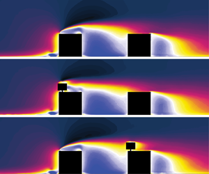
Figure 6 shows the streamwise velocity fields  $U_T/U_\infty$ for the six turbine positions. A wake behind the turbine can be observed in the flow fields, more prominently on the second cube. Studying this would be interesting for the potential placement of further turbines downstream. However, the focus in this study is on the upstream flow, as this is what influences the turbine performance.

Figure 6. Streamwise velocity fields with the wind turbine mounted at different streamwise positions along the centreline. Note that only every 20th vector is displayed to avoid clutter and all velocity vectors are scaled to be of uniform length, only representing the direction of flow.
Looking at the velocity vectors, it is apparent that at position 1F, the turbine entrains fluid from below as a result of the upstream blockage of the cube. This effect is increased by the presence of the turbine, which can be seen in table 1 by comparing the average skew angle  $\tilde {\gamma }$ upstream of the turbine for the flow field with and without the turbine. Note that $\tilde {\gamma }=0$ indicates no motion in the wall-normal direction, while positive $\tilde {\gamma }$-values indicate upward motion. At 1C the turbine is partly submerged in the recirculation bubble caused by the flow separation at the windward edge of the cube. The upper part of the turbine also experiences accelerated flow from above. This effect is increased by the presence of the turbine, which leads to a decreased $\tilde {\gamma }$. The turbulence intensity $\sqrt {\tilde {k}_{2D,T}}/U_\infty$ is increased by $6.4\,\%$ and $8.3\,\%$ for 1F and 1C, respectively. At 1B, the turbine is almost fully submerged in the recirculation zone. It encounters highly turbulent and chaotic flow, illustrated by an average incoming turbulence intensity $\sqrt {\tilde {k}_{2D,T}}/U_\infty$ of $18.9\,\%$ and strong variations in the skew angle. Only at the very top of the turbine is accelerated fluid entrained. The presence of the turbine only increases the turbulence intensity by ${\rm \Delta} \sqrt {\tilde {k}_{2D}}/U_\infty =0.6\,\%$.
On the second cube the turbine entrains high-speed fluid from the reattaching flow from above. This effect is most prominent at 2F. It is amplified by the presence of the turbine, indicated by increasingly negative  $\tilde {\gamma }$ for 2F, 2C and 2B. The flow from above the recirculation bubble is mixed with the wake of the first cube, leading to a significantly reduced magnitude of $\tilde {U}$ compared with $U_\infty$. Moving downstream on the second cube the flow recovers successively. This results in higher velocities and a reduced $\tilde {\gamma }$ towards the back of the second cube. The presence of the turbine reduces the difference in $\tilde {U}/U_\infty$ and $\sqrt {\tilde {k}_{2D}}/U_\infty$ between 2C and 2B, with the bigger change occurring from 2F to 2C. In general, the presence of the turbine slightly decreases the high turbulence intensities experienced on cube 2 by $0.7\,\% l \leqslant {\rm \Delta} \sqrt{\tilde{k}_{2D}}/U_\infty \leqslant\, 1.6\%$.
To illustrate further how the wind turbine changes the flow field at the different positions a differential velocity field  ${\rm \Delta} U / U_\infty$ generated by subtracting the velocity field of the empty cubes is plotted in figure 7; ${\rm \Delta} U = U_T-U_C$, where $U_T$ is the streamwise velocity field including the turbine and $U_C$ is the streamwise velocity field of the empty cubes. Here, $U_\infty$ is taken from the velocity field without the turbine. At positions 1F and 1C the turbine is placed in flow with a significant upward velocity component, as illustrated by figure 4(b), the velocity vectors in figure 6(a,b) and the skew angles in table 1. This creates an upwards deflected wake behind the turbine, visible in figure 7(a,b). At 1F the turbine also accelerates the flow below its wake, due to the disturbance of the recirculation bubble on top of the first cube. The turbine at 1B does not have a significant wake downstream of the turbine, due to the low velocities upstream of it. The turbine wake grows in magnitude and size with increasing downstream position on the second cube, as the flow upstream recovers. Detailed descriptions of VAWT wake characteristics can be found in Reference Shamsoddin and Porté-AgelShamsoddin and Porté-Agel (2014), Reference Rolin and Porté-AgelRolin and Porté-Agel (2018) and Reference Shamsoddin and Porté-AgelShamsoddin and Porté-Agel (2020).

Figure 7. Velocity difference caused by the presence of the wind turbine at different streamwise positions along the centreline.
More important for the turbine performance is the flow upstream of the turbine and this study reveals contrasting effects depending on the turbine position. At 1F the turbine shows a classical upstream blockage effect, where the streamwise velocity is slowed down by the presence of the turbine. It experiences a 27.5 % lower velocity than the flow field on the empty cubes would suggest. While the turbine at position 1B generates a similar upstream blockage at the top of the blade, overall the turbines at positions 1B and 1C have the opposite effect on the flow immediately upstream. Both turbines are partly placed in the recirculation bubble on top of the first cube. By virtue of obstructing the dominant reverse flow in this region, their presence causes more high-momentum fluid to enter the turbine area. This leads to a relative velocity surplus upstream of the turbines of 14.6 % and 132 % for 1C and 1B, respectively (table 1). This is a result that shows an impact of the turbine on the flow field that goes beyond established wind turbine blockage effects. Note the extreme relative increase on the back position is due to a very low  $\tilde {U}_C$ here. The trend is clear for both positions.
The turbines on the second cube again show more classical behaviour, causing an upstream blockage that slows down the flow by 30 % to 35 %. The flow is less skewed but more turbulent than on cube 1, which leads to enhanced deceleration of the flow upstream of the turbine. To determine the influence of those two factors rigorously would require a separate examination in a different set-up, which is outside the present scope and left for future investigations.
A more detailed analysis of the inflow at the turbine positions is shown in figure 8, where the histograms of the streamwise velocity along the blade height of the turbine  $h_T$, 0.05 $d_T$ upstream of the turbine are plotted. This is compared for the flow field $U_C$ without a turbine and for the flow fields $U_T$ including the turbine at various positions. It is apparent that the wind turbine encounters a wide range of inflow at the different turbine positions. The velocity profile is sheared at all positions, with strong gradients at positions 1C and 1B (figure 8b,c,e,f). The turbulent fluctuations increase on the first cube when moving the turbine downstream, indicated by wider histograms throughout $h_T$, while they decrease on cube 2, where the fluctuations are higher overall. The impact of the turbine on the incoming flow is visible at all positions, but is more prominent on the first cube. This is likely due to the fact that it is placed partly in a region of separating flow with high velocity gradients, whereas on cube 2 a recovering wake dominates, which is already a highly turbulent flow. At position 1F (figure 8a,d), the inflow without the turbine present is characterized by a low turbulence intensity $\sqrt {\tilde {k}_{2D,C}}/U_\infty =1.1\,\%$, indicated by a narrow histogram. The presence of the turbine reduces the streamwise velocity, most significantly in the centre, with the histograms showing large tails towards low velocities. This is also partly observed at the top of the turbine for 1C (figure 8b,e). Below that, the region of high shear is stretched and pushed down towards the lower part of the turbine. Here it replaces a low speed region, leading to an overall surplus of velocity compared with the case without the turbine. At 1B (figure 8c,f) the shear region is stretched similarly, diminishing the region of predominantly negative velocities. On the second cube the shape of the velocity profiles and width of the histograms do not change much in the presence of the turbine. The inflow is already highly turbulent with only a small gradient from top to bottom. A slight deficit around $z/h_T=0$ caused by the turbine can be observed, most prominent for position 2B (figure 8i,l). Overall the velocity is decreased on cube 2 for all positions, visible in the superimposed mean velocity profiles in figure 8. It is evident that the presence of the turbine has a significant impact on the flow phenomena across the system beyond blockage effects, which would result in significantly different power output from the real arrangement compared with predictions based off the system without the turbine alone. This is explicitly demonstrated in the next section.

Figure 8. Histograms of streamwise velocity  $U$ along the turbine blade immediately (0.05 $d_T$) upstream of the turbine from the flow fields without ((a–c) and (g–i)) and with the turbine ((d–f) and (j–l)). Mean velocity profiles superimposed as white lines.
4. Wind turbine performance
The converted power was measured as described in § 2. Based on this the mechanical power the wind turbine produced was calculated, considering the friction losses. In such a manner,  $P_m$ was evaluated for the six different locations. The goal of this study was not to evaluate how well the wind turbine performs but rather to compare different wind turbine positions on a modelled building environment. To do this the power coefficient $C_P = P_m / (\frac 1 2 \rho U_\infty^3 A)$ was calculated based on the incoming velocity $U_\infty$ upstream of the cubes; $C_P$ is listed in table 2 along with the other performance parameters such as $\lambda$, $P_m$, $P_c$ and $P_f$. The control of the tip speed ratio was fixed between different measurement positions leading to slight variations between 0.62 and 0.78. The values are in line with expected values for Savonius-type turbines (Reference Akwa, Vielmo and PetryAkwa et al., 2012; Reference Aliferis, Jessen, Bracchi and HearstAliferis et al., 2019).
Table 2. Wind turbine performance parameters.  $C_P$ is calculated based on $P_m$.

The available power at the turbine positions is expressed through a power coefficient of the available power  $C_{P_a}={({1}/{2})\rho \tilde {U}^3 A}/{({1}/{2})\rho U_\infty ^3 A}={\tilde {U}^3}/{U_\infty ^3}$, in order to represent it in non-dimensional form. Figure 9 shows $C_P$ at the different turbine positions in comparison with $C_{P_a}$, based on the measured velocities $\tilde {U}$ at these locations for the set-up with and without the turbine. Maximum uncertainties for $C_P$ and $C_{P_a}$ of 8.8 % and 3.5 %, respectively, are plotted for all cases. As shown by (Reference Akwa, Vielmo and PetryAkwa et al. 2012) $C_P$ values for Savonius turbines are generally low compared with HAWT and very dependent on Reynolds number. From $Re_{d_T}=280\,000$ to $Re_{d_T}=140\,000$ they report a reduction of $C_P$ from 0.17 to 0.13. In the present study $Re_{d_T}$ is almost an order of magnitude smaller at $Re_{d_T}=32\,000$, thus explaining the low $C_P$ values observed here. Of the positions tested, $C_P$ is at a maximum for the positions 1F and 1C, with a significant reduction in power as one moves towards the back of the cube (1B). On the second cube the extracted power increases with streamwise position. The turbine performance on cube 2 is higher at all positions compared with 1B but always remains below 1F and 1C. This suggests the outside positions, farthest away from the other building to be ideal in this configuration with one of the buildings directly downstream of the other and no other substantial obstructions in close proximity. However, the performance difference between this location and the centre of the cubes is small. Considering varying wind directions in reality and potentially multiple neighbouring buildings, the centre position offers a good balance of robustness and performance.

Figure 9. Analysis of the wind turbine performance at different positions based on the available power with and without the turbine ( $C_{P_{a,T}}$ and $C_{P_{a,C}}$) and the measured mechanical power ( $C_P$). Uncertainty bars based on propagation of uncertainty of all contributing variables.
It is apparent that the available power measured in the presence of the turbine  $C_{P_{a,T}}$ shows a much better correlation with the measured performance compared with that predicted from the flow field alone. The correlation coefficient $r(C_P,\,C_{P_{a,T}}) ={\rm cov} (C_P,\,C_{P_{a,T}}) / \sigma _{C_P} \sigma _{C_{P_{a,T}}}$ is $97.7\,\%$. Considering only the flow field around the empty cubes leads to deviations in the estimated available power $C_{P_{a,C}}$. The gap between the estimated available power at positions 1F and 1C is significantly overestimated. $C_{P_{a,C}}$ at 2C and 2B exceed $C_{P_{a,C}}$ at 1C, which contrasts with the measured power output (see $P_m$ and $C_P$ in table 2). The correlation coefficient $r(C_P,\,C_{P_{a,C}})$ is only $70.7\,\%$. The reason for this discrepancy between $C_{P_{a,C}}$ and $C_{P_{a,T}}$, and the resulting $C_P$ is the influence the wind turbine has on the flow field (see § 3.3). At position 1F and for all turbine positions on cube 2 $C_{P_{a}}$ is negatively affected by the presence of the turbine, whereas at positions 1C and 1B $C_{P_{a}}$ is increased by adding the turbine. These diverging trends lead to significantly different power estimates when considering only the flow field around the empty cubes.
5. Conclusions
The wind resources for two model buildings in tandem formation were evaluated using a combination of flow field and performance measurements. A VAWT of the Savonius (drag) type was placed at six different streamwise locations along the centreline of the roofs of the two buildings. It was shown that the presence of the turbine substantially influences the flow field and the power production. This extends beyond established wind turbine blockage effects previously reported in the literature. An analysis of the available power based only on the flow field around the cubes at the supposed turbine location, but without the turbine, would change the conclusions significantly. The available power calculated from the flow field in the presence of the turbine was found to correlate well with the power produced by the turbine at the various positions. The trends from front to back position differed between the first and second cube. The highest power was measured at the front and centre position of the first cube with a large reduction towards the back of cube 1. On the second cube the power production was found to increase gradually from front to back, with values in-between the extremes measured on the first cube. On the first cube the separation of the flow at the windward edge was the dominant flow pattern. The presence of the turbine diminished the recirculation zone on top of the cube and thus increased the available power at the centre and back position. At the front position the turbine affected the available power negatively due to upstream blockage effects and increased turbulent fluctuations. The second cube experienced a recovering wake from cube 1, which led to increasing power production with increasing distance from the upstream cube. Similarly to the front position on cube 1, the power production was diminished by the presence of the turbine, due to its upstream blockage effect.
It has to be noted that these conclusions are specifically for the present set-up and size ratios. However, the observed effects are expected to remain relevant in different configurations with similar size ratios. Future studies should investigate the influence of the size ratios of turbine to building  $d_T/h$ and $h_T/h$, the distance between the buildings $s/h$ as well as the influence of a staggered arrangement, the wind direction and the influence of incoming turbulence. Nonetheless, the results provided here suggest that in this specific configuration the ideal position of the turbine is on the outer edge of the buildings, farthest from the other building. More generally, the central positions on both buildings offer a good compromise between performance and robustness to the possibility of adjacent buildings and variations in incoming flow angle.
Supplementary Material
Supplementary material are available at https://doi.org/10.1017/flo.2022.3.
Declaration of Interest
The authors report no conflict of interest.
Funding Statement
This research received no specific grant from any funding agency, commercial or not-for-profit sectors.
Author Contributions
Y.J., T.B. and R.J.H. created the research plan. Y.J. and R.B. designed and built the set-up and conducted all experiments. Y.J. performed the analysis and wrote the manuscript. All authors contributed to the editing of the manuscript.
Data Availability Statement
See supplementary material.
Ethical Standards
The research meets all ethical guidelines, including adherence to the legal requirements of the study country.


 Open access