


1. Introduction
In this paper, we deal with the following three important problems of training neural networks with mixed categorical and numerical features in supervised learning tasks:
-
How to construct a numerical representation of categorical features which is fed, together with the numerical features, into the hidden layers of a neural network,
-
Which architecture of a neural network we should build, in particular, how we should treat (concatenate) features of different types (in our case categorical and numerical features),
-
How we should initialize the weights and the bias terms of a neural network to guide the network towards a point in the surface of parameters where the network has a high predictive power and good generalization properties.
There are many possible approaches to these problems. We present an approach inspired by autoencoders.
Neural networks have recently gained a lot of attention in actuarial science. In particular, Noll et al. (Reference Noll, Salzmann and Wüthrich2019) and Ferrario et al. (Reference Ferrario, Noll and Wüthrich2020) were among the first to discuss applications of neural networks to actuarial non-life insurance pricing problems and compared neural networks with generalized linear models. The current approach to supervised learning tasks in actuarial data science is to build a neural network where entity embeddings for categorical features are used. Entity embeddings were introduced by Guo and Berkhahn (Reference Guo and Berkhahn2016) in the machine learning literature to help neural networks to deal with sparse categorical data of high dimension. They were first promoted by Richman (Reference Richman2021), Noll et al. (Reference Noll, Salzmann and Wüthrich2019) and Ferrario et al. (Reference Ferrario, Noll and Wüthrich2020) in actuarial data science and they were further developed by Blier-Wong et al. (Reference Blier-Wong, Baillargeon, Cossette, Lamontagne and Marceau2021), Kuo and Richman (Reference Kuo and Richman2021) and Shi and shi (Reference Shi and Shi2022). An entity embedding, as part of a neural network for a supervised learning task, is learned separately for each categorical feature and allows us to derive a real-value representation of a categorical feature in a low-dimensional space. The numerical representations of the categorical features are concatenated with the numerical features and they are fed together as input into hidden layers of a neural network. The weights of the entity embeddings are learned together with all other parameters of the neural network, and the objective is to minimize a loss appropriate for a target response. All weights and bias terms of the network are initialized with random values from uniform distributions, and the back propagation algorithm is used to learn the parameters of the network. To the best of our knowledge, the architecture of a neural network described above is the only architecture of a neural network investigated to date for actuarial applications. In particular, other numerical representations of categorical features have not been tested as inputs to neural networks. In addition, advances in training algorithms for neural networks have not been discussed in actuarial data science. The only distinct training algorithm was proposed by Merz and Wüthrich (Reference Merz and Wüthrich2019) and Schelldorfer and Wüthrich (Reference Schelldorfer and Wüthrich2019) who promoted the Combined Actuarial Neural Network (CANN). The goal of this paper is to challenge the current dominant approach to supervised learning tasks in actuarial data science with a new architecture of a neural network, in particular, with a new numerical representation of categorical features and with a new training algorithm.
It is known that in order to achieve a high predictive power of a neural network, the input to the network should contain the most important information for the supervised learning task under consideration. A highly informative input can be effectively pre-processed in hidden layers of the network to provide good predictions of the response. It has been shown in the machine learning literature that non-linear autoencoders, in particular, denoising autoencoders, built with neural networks, can capture the main factors of variation in the input and detect key characteristics of the multivariate and high-dimensional distribution of the input. As a result, representations of features derived using (denoising) autoencoders, learned in unsupervised learning tasks, can improve the predictive power of regression models if these representations are used as inputs to neural networks to predict the response, see for example Vincent et al. (Reference Vincent, Larochelle, Bengio and Manzagol2008) and (Reference Vincent, Larochelle, Lajoie, Bengio and Manzagol2010).
Autoencoders without noise for numerical data have been investigated in actuarial data science. The benefits of autoencoders without noise in supervised and unsupervised learning tasks have been demonstrated by Gao and Wüthrich (Reference Gao and Wüthrich2018), Hainaut (Reference Hainaut2018), Rentzmann and Wüthrich (Reference Rentzmann and Wüthrich2019), Blier-Wong et al. (Reference Blier-Wong, Baillargeon, Cossette, Lamontagne and Marceau2021, Reference Blier-Wong, Cossette, Lamontagne and Marceau2022), Miyata and Matsuyama (Reference Miyata and Matsuyama2022) and Grari et al. (Reference Grari, Charpentier, Lamprier and Detyniecki2022). To the best of our knowledge, autoencoders for categorical features are less common in actuarial data science. The only exception we are aware of is the paper by Lee et al. (Reference Lee, Manski and Maiti2019) in which the authors discuss how to build word embeddings, which are similar to but are not exactly autoencoders for categorical data in the meaning investigated in this paper.
The first contribution of this paper is that we investigate different types of autoencoders for categorical data. We demonstrate that we can benefit from non-linear autoencoders built with neural networks when the purpose is to derive informative representations of categorical features. We show that an autoencoder for categorical features should be of a different type than an autoencoder for numerical features. Most importantly, we deduce that the best autoencoder for categorical features, which extracts the most important information from the vector of categorical features, implies a different numerical representation of categorical features than the representation from entity embeddings currently used in supervised learning tasks in actuarial data science. From our experiments, we conclude that we should learn one numerical representation for all categorical features, rather than multiple representations for each separate feature, to build a more robust and informative representation of the categorical data. The other, and our main contribution, is that we use a joint numerical representation of categorical features, together with all other numerical features, as the input to the hidden layers of a neural network trained to predict a target response. In other words, we introduce a new architecture of a neural network with mixed categorical and numerical features for the supervised learning tasks. The change in the architecture compared to the current approach is that all one-hot encoded categorical features are transformed with one embedding into a real-value representation in a low-dimensional space and the joint representation of the categorical features is then concatenated with the numerical features. Finally, we fine-tune the numerical representation of the categorical features from a proper autoencoder by training its weights together with all other parameters of the neural network. Hence, the autoencoder for the categorical data is only used to derive an initial representation of the categorical features. This approach is known in the machine learning literature as pre-training of layers with autoencodeders, see Vincent et al. (Reference Vincent, Larochelle, Bengio and Manzagol2008), Erhan et al. (Reference Erhan, Bengio, Courville, Manzagol, Vincent and Bengio2010, Reference Erhan, Manzagol, Bengio, Bengio and Vincent2009) and Vincent et al. (Reference Vincent, Larochelle, Lajoie, Bengio and Manzagol2010). Hence, we pre-train the joint embedding for categorical features in a neural network for a supervised learning task with our autoencoder for categorical data. From Erhan et al. (Reference Erhan, Manzagol, Bengio, Bengio and Vincent2009) and (Reference Erhan, Bengio, Courville, Manzagol, Vincent and Bengio2010), we know that pre-training other layers of the neural network is also beneficial, and this can be achieved with an autoencoder for numerical data. We use both autoencoders, without noise and denosing autoencoders, in this research.
The benefits of using (denosing) autoencoders for pre-training layers of neural networks have been demonstrated in the literature (see the papers referred to above). In comparison to these papers:
-
We perform our experiments with categorical data, instead of binary data, which means that we use a different autoencoder and a different type of a corruption process for the denoising autoencoder,
-
We perform our experiments with Poisson distributed data and the Poisson deviance loss, which is the most common loss function in actuarial data science, instead of the mean square loss and the cross-entropy loss commonly used in the machine learning literature,
-
We propose and validate a new architecture of a neural networks, with a joint embedding for all categorical features, for the supervised learning tasks. This has not been considered to date in actuarial data science,
-
We propose to scale appropriately the representation of the categorical features from an autoencoder for categorical data before an autoencoder for numerical data is built to pre-train the first hidden layer of a neural network. This improves significantly the approach to supervised learning tasks with our new architecture,
-
We compare various initialization techniques and we show that pre-training of layers of a neural network with non-linear and over-complete/denoising autoencoders produces much better results than applications of classical linear and under-complete autoencoders without noise (MCA, PCA),
-
We investigate the balance property, the bias and the stability of the predictions which are crucial for actuarial pricing.
The main conclusion of this paper is that we can improve the current approach to modelling categorical features in supervised learning tasks, which uses separate entity embeddings, and the training algorithm, which randomly initializes the parameters of the neural network. The proposal is to change the architecture of the network by using a different numerical representation of the categorical features, learned with a joint embedding, and initialize the layers of the network, in particular, the joint embedding and the first hidden layer, with representations learned with (denosing) autoencoders in unsupervised learning tasks.
This paper is structured as follows. In Section 2, we present the general setup for neural networks and our numerical experiments. In Section 3, we discuss autoencoders for categorical and numerical features. In Section 4, we focus on training neural networks with mixed categorical and numerical features. Details of our experiments and some additional results are presented in the Online Supplement. The R codes for training our categorical autoencoders are available on https://github.com/LukaszDelong/Autoencoders.
2. General setup
We assume that we have a data set consisting of $(y_i,{\boldsymbol{{x}}}_i)_{i=1}^n$
where
$(y_i,{\boldsymbol{{x}}}_i)_{i=1}^n$
where $y_i$
describes the one-dimensional response for observation i and
$y_i$
describes the one-dimensional response for observation i and ${\boldsymbol{{x}}}_i=(x_{1,i},..,x_{j,i},...,x_{d,i})^{\prime}$
is a d-dimensional vector of features which characterizes the observation. We may omit the index i, which indicates the observation, and simply use
${\boldsymbol{{x}}}_i=(x_{1,i},..,x_{j,i},...,x_{d,i})^{\prime}$
is a d-dimensional vector of features which characterizes the observation. We may omit the index i, which indicates the observation, and simply use $(y,{\boldsymbol{{x}}})$
. The vector
$(y,{\boldsymbol{{x}}})$
. The vector ${\boldsymbol{{x}}}$
consists of mixed categorical and numerical features. We assume that we have c categorical features and
${\boldsymbol{{x}}}$
consists of mixed categorical and numerical features. We assume that we have c categorical features and $d-c$
numerical features.
$d-c$
numerical features.
The categorical features are first one-hot encoded. Let $x_j$
denote a categorical feature with
$x_j$
denote a categorical feature with $m_j$
different labels
$m_j$
different labels $\left\{a^j_1,...,a^j_{m_j}\right\}$
. This categorical feature is transformed into a
$\left\{a^j_1,...,a^j_{m_j}\right\}$
. This categorical feature is transformed into a $m_j$
-dimensional vector of zeros and one:
$m_j$
-dimensional vector of zeros and one:
 \begin{eqnarray*}x_{j} \mapsto {\boldsymbol{{x}}}^{cat}_{j}=\big(x_{j_1},...,x_{j_{m_j}}\big)^{\prime}=\big(\mathbf{1}\{x_{j}=a^j_1\},...,\mathbf{1}\{x_{j}=a^j_{m_j}\}\big)^{\prime}\in {\mathbb{R}}^{m_j}.\end{eqnarray*}
The dimension of the vector of features ${\boldsymbol{{x}}}=\big(({\boldsymbol{{x}}}^{cat})^{\prime},({\boldsymbol{{x}}}^{num})^{\prime}\big)^{\prime}=\big(({\boldsymbol{{x}}}_{1}^{cat})^{\prime},...,({\boldsymbol{{x}}}_{c}^{cat})^{\prime},x_{c+1},...,x_{d}\big)^{\prime}$
becomes
${\boldsymbol{{x}}}=\big(({\boldsymbol{{x}}}^{cat})^{\prime},({\boldsymbol{{x}}}^{num})^{\prime}\big)^{\prime}=\big(({\boldsymbol{{x}}}_{1}^{cat})^{\prime},...,({\boldsymbol{{x}}}_{c}^{cat})^{\prime},x_{c+1},...,x_{d}\big)^{\prime}$
becomes $\sum_{j=1}^{c}m_j+d-c$
. As far as the numerical features are concerned, we assume that each numerical feature takes its values from
$\sum_{j=1}^{c}m_j+d-c$
. As far as the numerical features are concerned, we assume that each numerical feature takes its values from $[\!-\!1,1]$
, that is min–max scaler transformations are applied to the numerical features on the original scale.
$[\!-\!1,1]$
, that is min–max scaler transformations are applied to the numerical features on the original scale.
In general, we use neural networks with $M \in {\mathbb N}$
hidden layers and
$M \in {\mathbb N}$
hidden layers and $q_m\in {\mathbb N}$
neurons in each hidden layer
$q_m\in {\mathbb N}$
neurons in each hidden layer $m=1,\ldots,M$
. The network layers are defined with the mappings:
$m=1,\ldots,M$
. The network layers are defined with the mappings:
 \begin{eqnarray}{\boldsymbol{{z}}} \in {\mathbb R}^{q_{m-1}}\;\mapsto\;\theta^{m}({\boldsymbol{{z}}})&=&\big(\theta^{m}_1({\boldsymbol{{z}}}),\ldots,\theta^{m}_{q_m}({\boldsymbol{{z}}})\big)^{\prime}\in {\mathbb R}^{q_m},\quad m=1,\ldots,M, \end{eqnarray}
 \begin{eqnarray} {\boldsymbol{{z}}} \in {\mathbb R}^{q_{m-1}}\;\mapsto\;\theta^{m}_{r}({\boldsymbol{{z}}})&=&\chi^m\big(b_r^m+\langle{\boldsymbol{{w}}}^{m}_r,{\boldsymbol{{z}}}\rangle\big),\quad r=1,\ldots,q_m,\end{eqnarray}
where $\chi^m\;:\;{\mathbb R} \to {\mathbb R}$
denotes an activation function,
$\chi^m\;:\;{\mathbb R} \to {\mathbb R}$
denotes an activation function, ${\boldsymbol{{w}}}^m_r \in {\mathbb R}^{q_{m-1}}$
denotes the network weights,
${\boldsymbol{{w}}}^m_r \in {\mathbb R}^{q_{m-1}}$
denotes the network weights, $b^m_r \in {\mathbb R}$
denotes the bias term, and
$b^m_r \in {\mathbb R}$
denotes the bias term, and $\langle \cdot , \cdot \rangle$
denotes the scalar product in
$\langle \cdot , \cdot \rangle$
denotes the scalar product in ${\mathbb R}^{q_{m-1}}$
. By
${\mathbb R}^{q_{m-1}}$
. By $q_0$
we denote the dimension of the input vector to the network. The mapping:
$q_0$
we denote the dimension of the input vector to the network. The mapping:
 \begin{eqnarray}{\boldsymbol{{z}}} \in {\mathbb R}^{q_{0}}\; \mapsto \Theta^{M+1}({\boldsymbol{{z}}})=\big(\Theta_1^{M+1}({\boldsymbol{{z}}}),\ldots,\Theta_{q_{M+1}}^{M+1}({\boldsymbol{{z}}})\big)^{\prime} \in {\mathbb R}^{q_{M+1}},\end{eqnarray}
with a composition of the network layers $\theta^1, \ldots, \theta^M$
, and the components:
$\theta^1, \ldots, \theta^M$
, and the components:
 \begin{eqnarray*}{\boldsymbol{{z}}}\;\mapsto\;\Theta_r^{M+1}({\boldsymbol{{z}}})=b_r^{M+1}+\Big\langle{\boldsymbol{{w}}}_r^{M+1},\left(\theta^{M}\circ\cdots\circ\theta^1\right)({\boldsymbol{{z}}})\Big\rangle,\quad r=1,\ldots,q_{M+1},\end{eqnarray*}
gives us the prediction from the network in the output layer $M+1$
of dimension
$M+1$
of dimension $q_{M+1}$
based on the input vector
$q_{M+1}$
based on the input vector ${\boldsymbol{{z}}}$
. The output (2.3) returns the prediction with the linear activation function, and this prediction can be transformed with appropriate non-trainable and non-linear mapping if this is required for an application. If we set
${\boldsymbol{{z}}}$
. The output (2.3) returns the prediction with the linear activation function, and this prediction can be transformed with appropriate non-trainable and non-linear mapping if this is required for an application. If we set $M=0$
in (2.1)–(2.2), then we assume that the input vector is just linearly transformed to give the prediction in the output layer of dimension
$M=0$
in (2.1)–(2.2), then we assume that the input vector is just linearly transformed to give the prediction in the output layer of dimension $q_1$
and, in this case, the components in (2.3) are given by
$q_1$
and, in this case, the components in (2.3) are given by
 \begin{eqnarray*}{\boldsymbol{{z}}}\;\mapsto\;\Theta_r^{1}({\boldsymbol{{z}}})=b_r^{1}+\big\langle{\boldsymbol{{w}}}_r^{1},{\boldsymbol{{z}}}\big\rangle,\quad r=1,\ldots,q_{1}.\end{eqnarray*}
In our numerical experiments, we use the data set freMTPL2freq, which is included in the R package CASdatasets. The data set has 678,013 observations from insurance policies. The response Y describes the number of claims per policy. Each policy has nine features and an exposure: $({\boldsymbol{{x}}},Exp)$
. This data set is extensively studied by Noll et al. (Reference Noll, Salzmann and Wüthrich2019), Schelldorfer and Wüthrich (Reference Schelldorfer and Wüthrich2019) and Ferrario et al. (Reference Ferrario, Noll and Wüthrich2020) in the context of applications of generalized linear models and neural networks to modelling the number of claims. We perform the same data cleaning and feature pre-processing as in these papers. For the purpose of our experiments, we work with the features presented in Table 1.
$({\boldsymbol{{x}}},Exp)$
. This data set is extensively studied by Noll et al. (Reference Noll, Salzmann and Wüthrich2019), Schelldorfer and Wüthrich (Reference Schelldorfer and Wüthrich2019) and Ferrario et al. (Reference Ferrario, Noll and Wüthrich2020) in the context of applications of generalized linear models and neural networks to modelling the number of claims. We perform the same data cleaning and feature pre-processing as in these papers. For the purpose of our experiments, we work with the features presented in Table 1.
Table 1. Features used in our experiments.

We consider a supervised learning task where the goal is to predict the number of claims for a policyholder characterized by $({\boldsymbol{{x}}},Exp)$
by estimating the regression function
$({\boldsymbol{{x}}},Exp)$
by estimating the regression function ${\mathbb{E}}[Y|{\boldsymbol{{x}}},Exp]$
. The prediction is constructed with the neural network described above and the one-dimensional output from the network (2.3) is transformed with the non-trainable and the non-linear exponential transformation:
${\mathbb{E}}[Y|{\boldsymbol{{x}}},Exp]$
. The prediction is constructed with the neural network described above and the one-dimensional output from the network (2.3) is transformed with the non-trainable and the non-linear exponential transformation:
 \begin{eqnarray}{\mathbb{E}}[Y|{\boldsymbol{{x}}},Exp]=e^{\log(Exp)+\Theta_1^{M+1}({\boldsymbol{{x}}})}.\end{eqnarray}
The parameters of the network are trained by minimizing the Poisson deviance loss function, see for example Noll et al. (Reference Noll, Salzmann and Wüthrich2019), Schelldorfer and Wüthrich (Reference Schelldorfer and Wüthrich2019) and Ferrario et al. (Reference Ferrario, Noll and Wüthrich2020). Our supervised learning task is solved with the help of unsupervised learning tasks where autoencoders are used.
3. Autoencoders
Let ${\boldsymbol{{x}}}$
denote a vector of (categorical, numerical, mixed) features of dimension p. An autoencoder consists of two functions:
${\boldsymbol{{x}}}$
denote a vector of (categorical, numerical, mixed) features of dimension p. An autoencoder consists of two functions:
 \begin{eqnarray*}\varphi\;:\; {\mathbb{R}}^p \mapsto {\mathbb{R}}^l,\quad \text{and} \quad \psi\;:\; {\mathbb{R}}^l \mapsto {\mathbb{R}}^p.\end{eqnarray*}
The mapping $\varphi$
is called the encoder, and
$\varphi$
is called the encoder, and $\psi$
is called the decoder. The mapping
$\psi$
is called the decoder. The mapping ${\boldsymbol{{x}}}\mapsto\varphi({\boldsymbol{{x}}})$
from the encoder gives an l-dimensional representation of the p-dimensional vector
${\boldsymbol{{x}}}\mapsto\varphi({\boldsymbol{{x}}})$
from the encoder gives an l-dimensional representation of the p-dimensional vector ${\boldsymbol{{x}}}$
. The mapping
${\boldsymbol{{x}}}$
. The mapping ${\boldsymbol{{z}}}\mapsto\psi({\boldsymbol{{z}}})$
from the decoder tries to reconstruct the p-dimensional vector
${\boldsymbol{{z}}}\mapsto\psi({\boldsymbol{{z}}})$
from the decoder tries to reconstruct the p-dimensional vector ${\boldsymbol{{x}}}$
from its l-dimensional representation
${\boldsymbol{{x}}}$
from its l-dimensional representation ${\boldsymbol{{z}}}=\varphi({\boldsymbol{{x}}})$
. We define the reconstruction function as
${\boldsymbol{{z}}}=\varphi({\boldsymbol{{x}}})$
. We define the reconstruction function as
 \begin{eqnarray*}\pi=\psi\circ\varphi \;:\;{\mathbb{R}}^p\mapsto{\mathbb{R}}^p.\end{eqnarray*}
For a data set with observations $({\boldsymbol{{x}}}_i)_{i=1}^n$
, the goal is to find the functions
$({\boldsymbol{{x}}}_i)_{i=1}^n$
, the goal is to find the functions $\varphi$
and
$\varphi$
and $\psi$
such that the reconstruction error as
$\psi$
such that the reconstruction error as
 \begin{eqnarray*}\frac{1}{n}\sum_{i=1}^{n}L(\pi({\boldsymbol{{x}}}_i),{\boldsymbol{{x}}}_i),\end{eqnarray*}
measured with a loss function L, is minimized. If we can find an autoencoder for which the reconstruction error is small, then we can claim that the encoder extracts the most important information from a multi-dimensional vector of features. Consequently, we can use the representation $\varphi({\boldsymbol{{x}}})$
, instead of
$\varphi({\boldsymbol{{x}}})$
, instead of ${\boldsymbol{{x}}}$
, as input to predict the response in our supervised learning task. The observed response y is not used in this approach when we train an autoencoder. We train autoencoders in a fully unsupervised fashion, but we will improve the representation based on the target y when we solve the supervised learning task.
${\boldsymbol{{x}}}$
, as input to predict the response in our supervised learning task. The observed response y is not used in this approach when we train an autoencoder. We train autoencoders in a fully unsupervised fashion, but we will improve the representation based on the target y when we solve the supervised learning task.
Linear autoencoders are well-known in statistics. By a linear autoencoder, we mean an autoencoder where both the functions $\varphi$
and
$\varphi$
and $\psi$
are linear. Classical examples of linear autoencoders include autoencoders built with Principal Component Analysis for numerical data and Multiple Correspondence Analysis for categorical data. We refer for example to Chapter 6.2 in Dixon et al. (Reference Dixon, Halperin and Bilokon2020) for the equivalence between the linear autoencoder built by minimizing the mean square reconstruction loss function and the representation built with the PCA algorithm. For MCA and its relation to PCA, we refer for example to Pagès (Reference Pagès2015) and Chavent et al. (Reference Chavent, Kuentz-Simonet, Labenne and Saracco2017).
$\psi$
are linear. Classical examples of linear autoencoders include autoencoders built with Principal Component Analysis for numerical data and Multiple Correspondence Analysis for categorical data. We refer for example to Chapter 6.2 in Dixon et al. (Reference Dixon, Halperin and Bilokon2020) for the equivalence between the linear autoencoder built by minimizing the mean square reconstruction loss function and the representation built with the PCA algorithm. For MCA and its relation to PCA, we refer for example to Pagès (Reference Pagès2015) and Chavent et al. (Reference Chavent, Kuentz-Simonet, Labenne and Saracco2017).
In this paper, we are interested in non-linear autoencoders where at least one of the functions $\varphi$
or
$\varphi$
or $\psi$
is non-linear. We use the notation (2.1)–(2.2) from the previous section. To build an autoencoder for the input
$\psi$
is non-linear. We use the notation (2.1)–(2.2) from the previous section. To build an autoencoder for the input ${\boldsymbol{{x}}}$
, we use a neural network with one hidden layer, that is
${\boldsymbol{{x}}}$
, we use a neural network with one hidden layer, that is $M=1$
. The dimension of the single hidden layer is set to
$M=1$
. The dimension of the single hidden layer is set to $q_1=l$
, and the dimensions of the input and the output are set to
$q_1=l$
, and the dimensions of the input and the output are set to $q_0=q_2=p$
. The activation function for the hidden layer depends on the type of data and is discussed in the sequel. The vector
$q_0=q_2=p$
. The activation function for the hidden layer depends on the type of data and is discussed in the sequel. The vector $(\theta^1_1({\boldsymbol{{x}}}),...,\theta^1_l({\boldsymbol{{x}}}))^{\prime}$
gives us the representation of the input
$(\theta^1_1({\boldsymbol{{x}}}),...,\theta^1_l({\boldsymbol{{x}}}))^{\prime}$
gives us the representation of the input ${\boldsymbol{{x}}}$
from the encoder. The vector
${\boldsymbol{{x}}}$
from the encoder. The vector $(\Theta^2_1({\boldsymbol{{x}}}),...,\Theta^2_p({\boldsymbol{{x}}}))^{\prime}$
, transformed with a non-trainable and non-linear function if required for the data, gives us the reconstruction of the input
$(\Theta^2_1({\boldsymbol{{x}}}),...,\Theta^2_p({\boldsymbol{{x}}}))^{\prime}$
, transformed with a non-trainable and non-linear function if required for the data, gives us the reconstruction of the input ${\boldsymbol{{x}}}$
predicted with the decoder. This means that
${\boldsymbol{{x}}}$
predicted with the decoder. This means that $\psi$
also includes a non-trainable and non-linear transformation of the output (2.3) from the network if such a transformation is required for application. Clearly, we could also build deep autoencoders with more hidden layers, but shallow autoencoders with one hidden layer are sufficient for our main application in Section 4.
$\psi$
also includes a non-trainable and non-linear transformation of the output (2.3) from the network if such a transformation is required for application. Clearly, we could also build deep autoencoders with more hidden layers, but shallow autoencoders with one hidden layer are sufficient for our main application in Section 4.
If $l<p$
, we construct under-complete autoencoders and we reduce the dimension of the input
$l<p$
, we construct under-complete autoencoders and we reduce the dimension of the input ${\boldsymbol{{x}}}$
. Linear autoencoders built with the PCA and MCA algorithms are examples of under-complete autoencoders. If we choose
${\boldsymbol{{x}}}$
. Linear autoencoders built with the PCA and MCA algorithms are examples of under-complete autoencoders. If we choose $l=p$
, then we can achieve a zero reconstruction error by learning the identity mapping. Interestingly, we can also learn over-complete autoencoders with
$l=p$
, then we can achieve a zero reconstruction error by learning the identity mapping. Interestingly, we can also learn over-complete autoencoders with $l>p$
, and denoising autoencoders are examples of over-complete autoencoders. In order to construct a denoising autoencoder with
$l>p$
, and denoising autoencoders are examples of over-complete autoencoders. In order to construct a denoising autoencoder with $l>p$
, we corrupt the input for the network. The objective for training a denoising autoencoder is to find the functions
$l>p$
, we corrupt the input for the network. The objective for training a denoising autoencoder is to find the functions $\varphi$
and
$\varphi$
and $\psi$
such that the reconstruction error:
$\psi$
such that the reconstruction error:
 \begin{eqnarray*}\frac{1}{n}\sum_{i=1}^{n}L(\pi(\tilde{{\boldsymbol{{x}}}}_i),{\boldsymbol{{x}}}_i),\end{eqnarray*}
measured with a loss function L, is minimized. This time, the input $\tilde{{\boldsymbol{{x}}}}$
is corrupted input
$\tilde{{\boldsymbol{{x}}}}$
is corrupted input ${\boldsymbol{{x}}}$
which is constructed by adding a noise to
${\boldsymbol{{x}}}$
which is constructed by adding a noise to ${\boldsymbol{{x}}}$
. It has been demonstrated in the machine-learning literature that denosing autoencoders are very good at extracting the most important information from a multi-dimensional vector of features, see for example Vincent et al. (Reference Vincent, Larochelle, Bengio and Manzagol2008) and (Reference Vincent, Larochelle, Lajoie, Bengio and Manzagol2010). We can also construct over-complete autoencoders using data without noise if a low number of epochs is used for training the autoencoder built with a neural network.
${\boldsymbol{{x}}}$
. It has been demonstrated in the machine-learning literature that denosing autoencoders are very good at extracting the most important information from a multi-dimensional vector of features, see for example Vincent et al. (Reference Vincent, Larochelle, Bengio and Manzagol2008) and (Reference Vincent, Larochelle, Lajoie, Bengio and Manzagol2010). We can also construct over-complete autoencoders using data without noise if a low number of epochs is used for training the autoencoder built with a neural network.
In the next two sections, we discuss autoencoders for numerical and categorical features.
3.1. Autoencoders for numerical features
As discussed in Introduction, autoencoders without noise for numerical features have been investigated in various actuarial applications. In this paper, we adopt the approach from Rentzmann and Wüthrich (Reference Rentzmann and Wüthrich2019). We use the hyperbolic tangent activation function in the hidden layer ( $\chi^1$
), reconstruct the input using the linear prediction:
$\chi^1$
), reconstruct the input using the linear prediction:
 \begin{eqnarray}{\boldsymbol{{x}}}\in{\mathbb{R}}^p\mapsto\hat{{\boldsymbol{{x}}}}=\pi({\boldsymbol{{x}}})=\left(\Theta_1^2({\boldsymbol{{x}}}),...,\Theta_p^2({\boldsymbol{{x}}})\right)^{\prime}\in{\mathbb{R}}^p,\end{eqnarray}
and use the mean square error loss function L to measure the reconstruction error between the prediction $\hat{{\boldsymbol{{x}}}}=\pi({\boldsymbol{{x}}})$
and the input
$\hat{{\boldsymbol{{x}}}}=\pi({\boldsymbol{{x}}})$
and the input ${\boldsymbol{{x}}}$
. We build a non-linear autoencoder since we use a non-linear activation function (the hyperbolic tangent) in the hidden layer. In contrast to Rentzmann and Wüthrich (Reference Rentzmann and Wüthrich2019), we allow for bias terms in the network since we use the min–max scaler transformation of the numerical features instead of zero mean and unit variance standardization. An example of the architecture of a neural network used in this paper to build an autoencoder for numerical features is presented in Figure 1.
${\boldsymbol{{x}}}$
. We build a non-linear autoencoder since we use a non-linear activation function (the hyperbolic tangent) in the hidden layer. In contrast to Rentzmann and Wüthrich (Reference Rentzmann and Wüthrich2019), we allow for bias terms in the network since we use the min–max scaler transformation of the numerical features instead of zero mean and unit variance standardization. An example of the architecture of a neural network used in this paper to build an autoencoder for numerical features is presented in Figure 1.
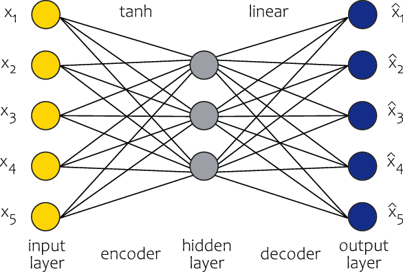
Figure 1. Architecture of the autoencoder for numerical features used in the paper.
As far as denoising autoencoders are concerned, we apply two types of corruption processes to distort the input, see for example Vincent et al. (Reference Vincent, Larochelle, Bengio and Manzagol2008), (Reference Vincent, Larochelle, Lajoie, Bengio and Manzagol2010):
-
Gaussian disturbance (gaussian): For each observation, $i=1,...,n$
, and each numerical feature in vector
${\boldsymbol{{x}}}_i$
, the original input is corrupted with the transformation
$x_{j,i}\mapsto\tilde{x}_{j,i}\sim N(x_{j,i},\sigma^2)$
.
$i=1,...,n$
, and each numerical feature in vector
${\boldsymbol{{x}}}_i$
, the original input is corrupted with the transformation
$x_{j,i}\mapsto\tilde{x}_{j,i}\sim N(x_{j,i},\sigma^2)$
. -
Masking to zero (zero): For each observation,
$i=1,...,n$
, and the fraction v of numerical features in vector
${\boldsymbol{{x}}}_i$
chosen at random, the original input is corrupted with the transformation
$x_{j,i}\mapsto\tilde{x}_{j,i}=0$
.


3.2. Autoencoders for categorical features
We consider two types of architecture of autoencoders for categorical features. Neither has been explored in the actuarial literature, although they appear, and versions of them appear, in many applications of machine learning methods in various fields.
-
1. Separate autencoders for each feature (Separate AEs): For categorical feature
$x_j$
with
$m_j$
different labels and its one-hot representation
${\boldsymbol{{x}}}_j^{cat}=(x_{j_1},...,x_{j_{m_j}})^{\prime}$
, we build a neural network (2.1)–(2.2) with
$M=1, q_0=m_j, q_1=l_j, q_2=m_j$
, where
$l_j$
is the required dimension of the representation of the categorical feature. Since we use the one-hot representation of
$x_j$
as the input to the network, there is no need to train bias terms in the hidden layer, so we set
$b^1_r=0$
for
$r=1,...,l_j$
. However, it is still beneficial to train bias terms in the output layer in order to match the output expressed with probabilities (see below). The linear activation function for
$\chi^1$
in the hidden layer is a natural choice here since the linear mappings
$\langle{\boldsymbol{{w}}}^{1}_r,{\boldsymbol{{x}}}^{cat}_j\rangle$
, for neurons
$r=1,...,l_j$
, yield unique constants for each label of the categorical feature, so there is no need to apply non-linear transformations to these constants. We reconstruct the input using the prediction: (3.2)where
\begin{eqnarray}{\boldsymbol{{x}}}_j^{cat}\in{\mathbb{R}}^{m_j}\mapsto\hat{{\boldsymbol{{x}}}}^{cat}_j=\pi({\boldsymbol{{x}}}_j^{cat})=\big(\pi_1({\boldsymbol{{x}}}_j^{cat}),...,\pi_{m_j}({\boldsymbol{{x}}}_j^{cat})\big)^{\prime}\in{\mathbb{R}}^{m_j},\end{eqnarray}
The soft-max activation function is applied to the output from the network (2.3) to derive the reconstructed input. The reconstruction function returns the probabilities that the reconstructed feature takes a particular label. The label with the highest predicted probability is the label predicted for the reconstructed feature. Since we now deal with a classification problem for the single categorical feature
\begin{eqnarray*}\pi_r({\boldsymbol{{x}}}_j^{cat})=\frac{e^{\Theta^2_r({\boldsymbol{{x}}}_j^{cat})}}{\sum_{u=1}^{m_j}e^{\Theta^2_u({\boldsymbol{{x}}}_j^{cat})}},\quad r=1,...,m_j.\end{eqnarray*}
$x_j$
, it is natural to use the cross entropy loss function L to measure the reconstruction error between the prediction
$\hat{{\boldsymbol{{x}}}}=\pi({\boldsymbol{{x}}})$
and the input
${\boldsymbol{{x}}}$
: (3.3)We build a non-linear autoencoder since we use a non-linear activation function (the soft-max function) in the output layer. The approach described above is applied to all categorical features in the data set. An example of the architecture of a neural network used in this paper to build the autoencoder of type Separate AEs for categorical features (with 2 and 3 labels) is presented in Figure 2.
\begin{eqnarray}L(\pi({\boldsymbol{{x}}}^{cat}_{j,i}),{\boldsymbol{{x}}}^{cat}_{j,i})=-\sum_{r=1}^{m_j}x^{cat}_{j_{r},i}\log\!\big(\pi_r({\boldsymbol{{x}}}^{cat}_{j,i})\big),\quad i=1,...,n.\end{eqnarray}
-
2. Joint autoencoder all features (Joint AE): We consider a vector of categorical features
$(x_1,...,x_c)$
with
$(m_1,...,m_c)$
different labels and their one-hot representations
${\boldsymbol{{x}}}^{cat}=\big(({\boldsymbol{{x}}}_1^{cat})^{\prime},...,$
$({\boldsymbol{{x}}}_c^{cat})^{\prime}\big)^{\prime}$
. Let
$\bar{m}_0=0$
and
$\bar{m}_j=\sum_{u=1}^j m_u$
for
$j=1,...,c$
. This time we build a neural network (2.1)–(2.2) with
$M=1, q_0=\bar{m}_c, q_1=l, q_2=\bar{m}_c$
, where l is the dimension of the required joint representation of all categorical features. We still set
$b^1_r=0$
for
$r=1,...,l$
, train bias terms in the output layer and apply the linear activation function in
$\chi^1$
. We reconstruct the input using the prediction: (3.4)where
\begin{eqnarray}{\boldsymbol{{x}}}^{cat}\in{\mathbb{R}}^{\bar{m}_c}\mapsto\hat{{\boldsymbol{{x}}}}^{cat}=\pi({\boldsymbol{{x}}}^{cat})&=&\big(\pi_1({\boldsymbol{{x}}}^{cat}),...,\pi_{\bar{m}_1}({\boldsymbol{{x}}}^{cat}), ...,\nonumber\\[5pt] &&\pi_{\bar{m}_{j-1}+1}({\boldsymbol{{x}}}^{cat}),...,\pi_{\bar{m}_j}({\boldsymbol{{x}}}^{cat}),...,\nonumber\\[5pt] &&\pi_{\bar{m}_{c-1}+1}({\boldsymbol{{x}}}^{cat}),...,\pi_{\bar{m}_c}({\boldsymbol{{x}}}^{cat})\big)^{\prime}\in{\mathbb{R}}^{\bar{m}_c},\end{eqnarray}
and
\begin{eqnarray*}\pi_r({\boldsymbol{{x}}}^{cat})=\frac{e^{\Theta^2_r({\boldsymbol{{x}}}^{cat})}}{\sum_{u=\bar{m}_{j-1}+1}^{\bar{m}_j}e^{\Theta^2_u({\boldsymbol{{x}}}^{cat})}},\quad r=\bar{m}_{j-1}+1,...,\bar{m}_j,\quad j=1,...,c,\end{eqnarray*}
$\pi_r({\boldsymbol{{x}}}^{cat})$
, for
$r=\bar{m}_{j-1}+1,...,\bar{m}_j$
, return probabilities that the categorical feature
$x_j$
takes a particular label among its
$m_j$
labels. The prediction of the label for
$x_j$
is the label with the highest predicted probability among
$\pi_r({\boldsymbol{{x}}}^{cat})$
. Clearly, we build a non-linear autoencoder. We remark that the soft-max activations functions are now applied to groups of neurons in the output layer from the network (2.3) which correspond to the labels of the categorical features. Hence, the decoder here returns probabilities in classification problems for all categorical features. This time all neurons in the layers of the autoencoder (before the soft-max transformations are applied) share the parameters of one neural network. By applying the Separate AEs, we independently solve multiple classification problems for our categorical features with separate autoencoders, whereas by applying the Joint AE, we jointly solve multiple classification problems for our categorical features with one autoencoder. Such an approach is called multi-task learning in machine learning, see for example Caruana (Reference Caruana1997) and Ruder (Reference Ruder2017). We use the cross entropy loss function L to measure the reconstruction error between prediction
$\hat{{\boldsymbol{{x}}}}=\pi({\boldsymbol{{x}}})$
and input
${\boldsymbol{{x}}}$
: (3.5)An example of the architecture of type Joint AE is presented in Figure 3.
\begin{eqnarray}L(\pi({\boldsymbol{{x}}}_i^{cat}),{\boldsymbol{{x}}}_i^{cat})=-\sum_{j=1}^c\sum_{r=1}^{m_j}x^{cat}_{j_{r},i}\log\!\big(\pi_r({\boldsymbol{{x}}}^{cat}_i)\big),\quad i=1,...,n.\end{eqnarray}


Figure 2. Architecture of the autoencoder of type Separate AEs for categorical features.

Figure 3. Architecture of the autoencoder of type Joint AE for categorical features.
In order to build denosing autoencoders, we apply the following corruption processes for categorical features:
-
For each observation,
$i=1,...,n$
, and a fraction v of categorical features in vector
${\boldsymbol{{x}}}_i$
chosen at random, the original input is corrupted with the transformations: -
Sampling a new label (sample): The original input is corrupted with the transformation
$x_{j,i}\mapsto\tilde{x}_{j,i}\sim \hat{F}_{x_j}$
and one-hot encoded with
$\tilde{x}_{j,i}\mapsto \tilde{{\boldsymbol{{x}}}}^{cat}_{j,i}$
, where
$\hat{F}_{x_j}$
is the empirical distribution of the feature
$x_j$
in the data set. This corruption process can be seen as an extension of the salt-and-pepper noise for binary data to categorical data, see for example Vincent et al. (Reference Vincent, Larochelle, Bengio and Manzagol2008, Reference Vincent, Larochelle, Lajoie, Bengio and Manzagol2010) for the salt-and-pepper noise for binary data. -
Masking to zero (zero): The original input and its one-hot encoding are corrupted with the transformation
${\boldsymbol{{x}}}^{cat}_{j,i}\mapsto\tilde{{\boldsymbol{{x}}}}^{cat}_{j,i}=\mathbf{0}'$
, where
$\mathbf{0}$
is a vector of zeros. This corruption process is an analogue to the technique of masking applied to numerical features from Section 3.1.


We conclude this section with some remarks on the types of architecture of our autoencoders for categorical data:
-
(a) The approach with the Separate AEs has at least two disadvantages compared to the Joint AE. First, we have to train a number of autoencoders equal to the number of categorical features, which may be time-consuming. Secondly, and more importantly, we neglect possible dependencies between different categorical features when creating representations with separate and independent autoencoders. The second disadvantage is explored in Experiment 1 below. We consider the approach with the Separate AEs as a benchmark since it gives us a representation of categorical data which matches the representation of categorical data learned with entity embeddings in supervised learning tasks.
-
(b) If the categorical features are binary features, then our approach with the Joint AE is aligned with the approach for binary data used by Vincent et al. (Reference Vincent, Larochelle, Bengio and Manzagol2008, Reference Vincent, Larochelle, Lajoie, Bengio and Manzagol2010) in their experiments. For binary data, autoencoders which coincide with our Joint AE are also used in Generative Adversarial Imputation Nets, see for example Yoon et al. (Reference Yoon, Jordon and Van der Schaar2018).
-
(c) Hespe (Reference Hespe2020) recommends a multi-task learning autoencoder for categorical data which agrees with our Joint AE. He also describes single-task learning autoencoders learned with loss functions different from the cross-entropy.
3.3. Experiment 1: the reconstruction ability of autoencoders
We compare the following four autoencoders for categorical data:
-
Separate AEs,
-
Joint AE,
-
MCA — we build a linear autoencoder with the classical MCA algorithm, that is instead of training a neural network, we apply Generalized Singular Value Decomposition (GSVD) to a matrix with centered one-hot encoded categorical features, see Pagès (Reference Pagès2015) and Chavent et al. (Reference Chavent, Kuentz-Simonet, Labenne and Saracco2017),
-
MCA as non-linear PCA — we build a non-linear autoencoder for numerical data, the one described in Section 3.1, on linearly transformed one-hot encoded categorial features. From Pagès (Reference Pagès2015) and Chavent et al. (Reference Chavent, Kuentz-Simonet, Labenne and Saracco2017), MCA is PCA on centered one-hot encoded categorical data transformed with linear mappings (GSVD). Instead of building a linear autoencoder, which is equivalent to the PCA algorithm, on linearly transformed centered one-hot encoded categorial features, we build a non-linear autoencoder with the hyperbolic tangent activation function in the single hidden layer by minimizing the mean square reconstruction error.
From the data set freMTPL2freq with 678,013 observations, we sample 100,000 observations. We work with a smaller data set to speed up the calculations. We limit our attention to categorical features and we consider the six categorical features from Table 1. Our data set with 100,000 observations is next split randomly into five data sets with 20,000 observations. We build our autoencoders on each of these five sets and report the average metric for these five sets evaluated at the training set. As the metric, we use the cosine similarity measure, but the findings also hold for example for the number of correct predictions. In this experiment, we only build under-complete autoencoders without noise, as this is sufficient to derive the key conclusions. We train our autoencoders with 15, 100 and 500 epochs. We do not differentiate between a training, a validation and a test set (we do not discuss possible over-fitting) since we are only interested in evaluating the reconstruction errors of the autoencoders. Details are presented in Section 1 in the Online Supplement.
The dimension of the data matrix with the one-hot encoded categorical features is 54. We consider a range of dimensions of the representation of the categorical features: $q_1=l=6,8,10,12,15,20,30$
. For the Separate AEs, we have to specify the number of neurons
$q_1=l=6,8,10,12,15,20,30$
. For the Separate AEs, we have to specify the number of neurons $l_j$
(the dimension of representation) for each feature j. We assume that the number of neurons l, which defines the global dimension of the representation for all categorical features, is split across the individual categorical features evenly, if possible, and if not possible, a larger number of neurons is allocated to a feature with a larger number of labels. For example if we choose
$l_j$
(the dimension of representation) for each feature j. We assume that the number of neurons l, which defines the global dimension of the representation for all categorical features, is split across the individual categorical features evenly, if possible, and if not possible, a larger number of neurons is allocated to a feature with a larger number of labels. For example if we choose $l=6$
, then we build representations of dimension 1 for each feature, if we choose
$l=6$
, then we build representations of dimension 1 for each feature, if we choose $l=12$
, then we build representations of dimension 2 for each feature, but if we choose
$l=12$
, then we build representations of dimension 2 for each feature, but if we choose $l=8$
, then we build representations of dimension 2 for Region and VehBrand (these two features have the two largest number of labels in the data set) and representations of dimension 1 for the remaining features.
$l=8$
, then we build representations of dimension 2 for Region and VehBrand (these two features have the two largest number of labels in the data set) and representations of dimension 1 for the remaining features.
We present the results in Figure 4. It is obvious that the cosine similarity increases with the number of neurons and the number of epochs. For the large number of epochs (500), for which we achieve the smallest reconstruction errors for all our autoencoders in terms of the loss functions minimized in the training process, the autoencoders Separate AEs and Joint AE are very similar in terms of their reconstruction power measured with the cosine similarity and they are much better than the remaining two autoencoders. The first conclusion confirms that categorical data have different intrinsic properties than numerical data, which are explored when a low-dimensional representation is built with an autoencoder, and categorical data should not be compressed with algorithms derived for numerical data (MCA is just PCA on linearly transformed data). The second conclusion is that for the low and the medium number of epochs (15, 100), especially for the low number of epochs, the performance of Joint AE is superior in terms of its ability to reconstruct the input from a low dimensional representation. In particular, our experiment shows that there are dependencies between the categorical features in the data set which are efficiently captured by the Joint AE at initial epochs (15 epochs) of the learning process of the autoencoder, and which cannot be captured by learning independent Separate AEs. Intuitively, dependencies between categorical features should allow the Joint AE to learn more robust and informative representations of categorical features and the Joint AE should lead to better reconstruction errors compared to the Separate AEs. For the low number of epochs (15) and a low dimension of the representation (6, 8, 10), the Joint AE is very similar to the MCA, but the performance of the Joint AE improves quickly when we increase the number of epochs. Clearly, we can benefit from non-linear autoencoders when the purpose is to derive informative representations of categorical features.

Figure 4. Cosine similarity measures for autoencoders for categorical data.
As discussed in Section 3, if we can find an autoencoder for which the reconstruction error is small, then we can say that the encoder extracts the most important information from a multi-dimensional vector of features. Our example points out that representations of categorical features built with the Separate AEs may not be optimal in terms of their robustness and informativeness, especially if we do not want to spend much time on training autoencoders with a large number of epochs. It is known that the predictive power of neural networks and their generalization properties in supervised learning tasks depend on providing a good representation of the available information for its efficient pre-processing in hidden layers before the final prediction of the response is constructed with the output. Since the Joint AE performs better than the Separate AEs in terms of providing a more robust and informative representation of categorical features, we may prefer to use the numerical representation of categorical features implied by the Joint AE, rather than the Separate AEs, as the input to neural networks built for supervised learning tasks. However, in all practical examples in actuarial data science to date, the numerical representation of categorical features which is fed into hidden layers of a neural network matches the representation from the Separate AEs. We have to use a different type of architecture of a neural network to use the representation from the Joint AE. This experiment may serve as a motivating example for what we present in the sequel.
4. Training neural networks with mixed categorical and numerical features
We now move to the main topic of this paper. Below, we discuss different approaches to training neural networks with mixed categorical and numerical features in supervised learning tasks. These approaches differ in the architecture of the neural network and initialization of the parameters of the neural network.
4.1. Architecture A1 with separate entity embeddings
Let us start by recalling the concept of an entity embedding developed by Guo and Berkhahn (Reference Guo and Berkhahn2016). An entity embedding for categorical feature $x_j$
is a neural network which maps the categorical feature
$x_j$
is a neural network which maps the categorical feature $x_j$
, with its one-hot representation
$x_j$
, with its one-hot representation ${\boldsymbol{{x}}}_j^{cat}$
, into a vector of dimension
${\boldsymbol{{x}}}_j^{cat}$
, into a vector of dimension $l_j$
:
$l_j$
:
 \begin{eqnarray*}{\boldsymbol{{x}}}^{cat}_{j}\in{\mathbb{R}}^{m_j} \mapsto {\boldsymbol{{x}}}^{ee}_{j}=(x^{ee}_{j_1},...,x^{ee}_{j_{l_j}})^{\prime}\in{\mathbb{R}}^{l_j},\end{eqnarray*}
where
 \begin{eqnarray*}x^{ee}_{j_r}=\langle{\boldsymbol{{w}}}^{ee}_r,{\boldsymbol{{x}}}^{cat}_j\rangle,\quad r=1,...,l_j.\end{eqnarray*}
With an entity embedding, each label, from the set of $m_j$
possible labels
$m_j$
possible labels $\{a_1,...,a_{m_j}\}$
of the categorical feature
$\{a_1,...,a_{m_j}\}$
of the categorical feature $x_j$
, can be represented with a vector in the space
$x_j$
, can be represented with a vector in the space ${\mathbb{R}}^{l_j}$
. The parameter
${\mathbb{R}}^{l_j}$
. The parameter $l_j$
is the dimension of the embedding for the categorical feature
$l_j$
is the dimension of the embedding for the categorical feature $x_j$
.
$x_j$
.
In Figure 5, we provide an example of the architecture of a neural network with mixed categorical and numerical features used in supervised learning tasks in actuarial data science. This architecture uses entity embeddings for categorial features and has been promoted by Richman (Reference Richman2021), Noll et al. (Reference Noll, Salzmann and Wüthrich2019) and Ferrario et al. (Reference Ferrario, Noll and Wüthrich2020). We present a simple example with two categorical features ${\boldsymbol{{x}}}^{cat}_1, {\boldsymbol{{x}}}^{cat}_2$
, with 3 and 2 levels, and two numerical features
${\boldsymbol{{x}}}^{cat}_1, {\boldsymbol{{x}}}^{cat}_2$
, with 3 and 2 levels, and two numerical features $x_3$
and
$x_3$
and $x_4$
. For
$x_4$
. For ${\boldsymbol{{x}}}^{cat}_1$
, we implement the entity embedding of dimension 2, and for
${\boldsymbol{{x}}}^{cat}_1$
, we implement the entity embedding of dimension 2, and for ${\boldsymbol{{x}}}^{cat}_2$
— the entity embedding of dimension 1. More generally, within (2.1)–(2.2), we define a neural network with Architecture 1 (A1):
${\boldsymbol{{x}}}^{cat}_2$
— the entity embedding of dimension 1. More generally, within (2.1)–(2.2), we define a neural network with Architecture 1 (A1):
-
For each categorical feature
$x_j$
,
$j=1,..,c$
, we build an entity embedding — a sub-network without hidden layers, that is
$M=0$
, where the input
${\boldsymbol{{z}}}={\boldsymbol{{x}}}^{cat}_j$
,
$q_0=m_j$
and the output
$q_1=l_j$
, -
Once all one-hot encoded categorical features are transformed with linear mappings of the entity embeddings, the outputs from the entity embeddings, that is the numerical representations of the categorical features, are concatenated with the numerical features to yield a new numerical vector of all features. This new vector is fed as the input into another sub-network with M hidden layers,
-
We build a sub-network with M hidden layers with neurons
$q_1,...,q_M$
and the hyperbolic tangent activation functions
$\chi^1,...,\chi^M$
in the hidden layers, where the input
${\boldsymbol{{z}}}=\big(({\boldsymbol{{x}}}^{ee}_1)^{\prime},...,({\boldsymbol{{x}}}^{ee}_c)^{\prime},x_{c+1},...,x_d\big)^{\prime}$
and
$q_0=\sum_{j=1}^cl_j+d-c$
, -
All weights of the network (including the weights of the entity embeddings) are initialized with values sampled from uniform distributions with the Xavier initialization, see Glorot and Bengio (Reference Glorot and Bengio2010), and the bias terms are initialized with zero.


Figure 5. Architecture of type A1 with separate entity embeddings.
The goal of this paper is to challenge A1 with a new architecture and a new training process of a neural network. The results from Experiment 1 provide us with arguments regarding how we could change A1. We can now clearly observe that the numerical representations of the categorical features learned with the entity embeddings in A1 matches, in their architectures, the numerical representations learned with the Separate AEs. From Section 3.3, we conclude that we could replace the numerical representations of the categorical features in A1 with the representation learned with the Joint AE. This leads us to introduce Architecture 2.
4.2. Architecture A2 with joint embedding
Instead of applying separate entity embeddings to each categorical feature, we now use a joint embedding for all categorical features. A joint embedding is understood here as a neural network with the following mapping:
 \begin{eqnarray*}{\boldsymbol{{x}}}^{cat}=(({\boldsymbol{{x}}}^{cat}_1)^{\prime},...,({\boldsymbol{{x}}}^{cat}_c)^{\prime})^{\prime}\in{\mathbb{R}}^{\bar{m}_c} \mapsto {\boldsymbol{{x}}}^{\tilde{ee}}=(x^{\tilde{ee}}_{1},...,x^{\tilde{ee}}_{l})^{\prime}\in{\mathbb{R}}^{l},\end{eqnarray*}
where
 \begin{eqnarray*}x^{\tilde{ee}}_{r}=\langle{\boldsymbol{{w}}}^{\tilde{ee}}_r,{\boldsymbol{{x}}}^{cat}\rangle,\quad r=1,...,l.\end{eqnarray*}
Parameter l is the dimension of the embedding for all categorical features $(x_1,...,x_c)$
. We expect that
$(x_1,...,x_c)$
. We expect that $l<l_1+...+l_c$
.
$l<l_1+...+l_c$
.
Our new architecture of a neural network with mixed categorical and numerical features where the categorical features are modelled with a joint embedding is presented in Figure 6. For ${\boldsymbol{{x}}}^{cat}_1,{\boldsymbol{{x}}}^{cat}_2$
, we implement a joint embedding of dimension 3—this is the only, but also a significant difference between the architectures in Figures 5 and 6. Within (2.1) and (2.2), we define a neural network with Architecture 2 (A2):
${\boldsymbol{{x}}}^{cat}_1,{\boldsymbol{{x}}}^{cat}_2$
, we implement a joint embedding of dimension 3—this is the only, but also a significant difference between the architectures in Figures 5 and 6. Within (2.1) and (2.2), we define a neural network with Architecture 2 (A2):
-
For all categorical features
$(x_1,...,x_c)$
, we build a joint embedding — a neural sub-network without hidden layers, that is
$M=0$
, where the input
${\boldsymbol{{z}}}={\boldsymbol{{x}}}^{cat}$
,
$q_0=\bar{m}_c$
and the output
$q_1=l$
, -
The next steps of building the network for predicting the response are the same as for A1.
-
We initialize all weights with the Xavier initialization and set the bias terms equal to zero, as for A1.


Figure 6. Architecture of type A2 with joint embedding.
We can observe that the numerical representation of the categorical features learned with the joint embedding in A2 matches, in its architecture, the representation learned with the Joint AE. We have already discussed the advantages of this representation in unsupervised learning tasks, which should also hold in supervised learning tasks. In addition, we can expect that by learning a joint embedding for all categorical features, we allow all categorical features, not only labels for a single categorical feature, to share the information about their impact on the response. As a result, we should be able to improve predictions of the response based on the experience collected from similar categorical features and their similar labels. Hence, the switch from A1 to A2 has intuitive foundations. To the best of our knowledge, A2 has not been considered to date in any actuarial data science problem.
4.3. Initialization of A1 and A2
The issue of initialization of parameters of neural networks has been noticed in actuarial data science. Under A1, Merz and Wüthrich (Reference Merz and Wüthrich2019) and Schelldorfer and Wüthrich (Reference Schelldorfer and Wüthrich2019) propose the Combined Actuarial Neural Network (CANN) approach to initialize a neural network with predictions from a GLM — we call this architecture and the training process A1_CANN. The idea is to add a skip connection to the output from the network with architecture A1. In mathematical terms, in A1 we use the prediction:
 \begin{eqnarray}\lambda_i=e^{\log(Exp_i)+\Theta_1^{M+1}\big((({\boldsymbol{{x}}}^{ee}_{1,i})^{\prime},...,({\boldsymbol{{x}}}^{ee}_{c,i})^{\prime},x_{c+1,i},...,x_{d,i})^{\prime}\big)},\quad i=1,...,n,\end{eqnarray}
whereas in A1_CANN we use the prediction:
 \begin{eqnarray}\lambda_i=e^{\log(Exp_i)+\eta^{GLM}_i+\Theta_1^{M+1}\big((({\boldsymbol{{x}}}^{ee}_{1,i})^{\prime},...,({\boldsymbol{{x}}}^{ee}_{c,i})^{\prime},x_{c+1,i},...,x_{d,i})^{\prime}\big)},\quad i=1,...,n,\end{eqnarray}
where $\eta^{GLM}_i$
denotes the prediction, on the linear scale, of the unit intensity (for exposure equal to one) from a Poisson GLM with a log link for observation i.
$\eta^{GLM}_i$
denotes the prediction, on the linear scale, of the unit intensity (for exposure equal to one) from a Poisson GLM with a log link for observation i.
In A1 and A2, we initialize the weights of the embeddings for the categorical features with the Xavier initialization. However, since autoencoders extract important information about features, we could initialize the weights of the embeddings with the weights from the encoder of the appropriate autoencoder and define the weights of the embeddings as non-trainable in the training process. This is reasonable, but may be sub-optimal for a supervised learning task since the representation of the categorical features learned with an autoencoder without the information about the response would be kept fixed. To improve the representation from an autoencoder, we should fine-tune it in a supervised learning task with a target response. In the machine learning literature, Erhan et al. (Reference Erhan, Bengio, Courville, Manzagol, Vincent and Bengio2010, Reference Erhan, Manzagol, Bengio, Bengio and Vincent2009) propose to pre-train layers of neural networks with denoising autoencoders, that is initialize neurons in layers of a neural network for a supervised learning task with representations of the neurons from denoising autoencoders built in unsupervised learning tasks for the input to the layers. We recover and modify their approach in this paper.
Apart from changing the architecture from A1 to A2, we initialize the weights and the bias terms in the joint embedding for the categorical feature and the first hidden layer in A2 with the weights and the bias terms from the representations of the neurons in the layers learned with autoencoders. From Erhan et al. (Reference Erhan, Bengio, Courville, Manzagol, Vincent and Bengio2010, Reference Erhan, Manzagol, Bengio, Bengio and Vincent2009), we know that the initialization procedure with autoencoders gives the largest gains in predictive power of a neural network when it is applied to initial layers of the network. We proceed in the following way:
-
We build an autoencoder of type Joint AE (denoted as the 1st AE) for the categorical input
$(x_1,...,x_c)$
using its one-hot representation
${\boldsymbol{{x}}}^{cat}=\big(({\boldsymbol{{x}}}^{cat}_1)^{\prime},...,({\boldsymbol{{x}}}^{cat}_c)^{\prime}\big)^{\prime}$
. To build a denoising autoencoder, we corrupt the categorical input with the sample or the zero transformation, see Section 3.2, -
We take the weights from the encoder of the 1st AE, denoted by
${\boldsymbol{{w}}}^{enc}_r=(w^{enc}_{r,1},...,w^{enc}_{r,\bar{m}_c}), r=1,...,l$
, and initialize the weights
${\boldsymbol{{w}}}^{\tilde{ee}}_r, r=1,...,l,$
of the joint embedding in A2 with these weights, -
We take the representation of the categorical features predicted by the 1st AE:
${\boldsymbol{{x}}}^{enc}=(x^{enc}_1,...,x^{enc}_l)^{\prime}$
with
$x^{enc}_{r}=\langle{\boldsymbol{{w}}}^{enc}_r,{\boldsymbol{{x}}}^{cat}\rangle, r=1,...,l$
, concatenate this vector with the vector of the numerical features
$(x_{c+1},...,x_d)^{\prime}$
and create a new vector of numerical features
${\boldsymbol{{z}}}=(({\boldsymbol{{x}}}^{enc})^{\prime},x_{c+1},...,x_d)^{\prime}$
, -
We build an autoencoder from Section 3.1 (denoted as the 2nd AE) for the numerical input
${\boldsymbol{{z}}}$
. The dimension of the representation to be learned for the
$(l+d-c)$
-dimensional vector
${\boldsymbol{{z}}}$
is equal to
$q_1$
, where
$q_1$
denotes the number of neurons used in the first hidden layer in the sub-network with M hidden layers, which is built for the input constructed by concatenating the representation from the joint embedding with the numerical features. To build a denoising autoencoder, we corrupt the numerical input with the gaussian or the zero transformation, see Section 3.1, -
We take the weights and the bias terms from the encoder of the 2nd AE and initialize the weights and the bias terms
$b^1_r, {\boldsymbol{{w}}}^1_r, r=1,...,q_1,$
in the first hidden layer in the sub-network with M hidden layers with these weights and the bias terms. -
All other weights are initialized with the Xavier initialization and the bias terms are initialized with zero.


The initialization procedure applied here also clarifies why we were only interested in building autoencoders with one hidden layer in Section 3. For A2, and any initialization of layers, we use the predictions:
 \begin{eqnarray}\lambda_i=e^{\log(Exp_i)+\Theta_1^{M+1}\big((({\boldsymbol{{x}}}_i^{\tilde{ee}})^{\prime},x_{c+1,i},...,x_{d,i})^{\prime}\big)},\quad i=1,...,n.\end{eqnarray}
The autoencoders, which are trained without the information about the response, are only used to derive initial values of the neurons in the two layers of A2. These initial values are next fine-tuned by training the whole neural network to predict the target response. When training an autoencoder, we are only interested in extracting the most important discriminatory factors in the multi-dimensional input vector, which are next improved and optimally transformed by taking into account the target response. Since in this application autoencoders are trained for a low number of epochs, in Experiment 1, we should only look at the results for epochs 15 and 100, which show clear advantages of the representation of categorical features learned with the Joint AE compared to the Separate AEs.
The third step above where we concatenate the numerical representation of the categorical features from the 1st AE with the other numerical features deserves attention. We propose a modification of the pre-training strategy of layers with autoencoders which has not been considered by Erhan et al. (Reference Erhan, Bengio, Courville, Manzagol, Vincent and Bengio2010, Reference Erhan, Manzagol, Bengio, Bengio and Vincent2009). It is known that the features, fed into a neural network, should live on the same scale in order to perform effective training of the network. We can easily control the numerical features and scale them to $[-1,1]$
, which is done before the training process is started. However, we cannot expect the numerical representation of the categorical features learned with the 1st AE, that is the values given by
$[-1,1]$
, which is done before the training process is started. However, we cannot expect the numerical representation of the categorical features learned with the 1st AE, that is the values given by $x_r^{enc}=\langle{\boldsymbol{{w}}}^{enc}_r,{\boldsymbol{{x}}}^{cat}\rangle, r=1,...,l$
, to yield predictions in
$x_r^{enc}=\langle{\boldsymbol{{w}}}^{enc}_r,{\boldsymbol{{x}}}^{cat}\rangle, r=1,...,l$
, to yield predictions in $[-1,1]$
. If the predictions from the encoder of the 1st AE live on a scale different from
$[-1,1]$
. If the predictions from the encoder of the 1st AE live on a scale different from $[-1,1]$
, which is the scale where the numerical features live, then the input to the 2nd AE and the input to the first hidden layer of the sub-network with M hidden layers will have features on different scales, and the training process of the neural networks may suffer from this inconsistency in scales. Fortunately, we can modify the weights and the bias terms of the encoder and the decoder of the 1st AE to keep the reconstruction error unchanged and have the representation of the categorical features in the desired scale. This is possible due to the linear activations functions assumed and the bias terms chosen to be trained in the output layer in the autoencoder of type Joint AE, before the soft-max functions are applied. In the encoder part of the Joint AE, we re-define the weights:
$[-1,1]$
, which is the scale where the numerical features live, then the input to the 2nd AE and the input to the first hidden layer of the sub-network with M hidden layers will have features on different scales, and the training process of the neural networks may suffer from this inconsistency in scales. Fortunately, we can modify the weights and the bias terms of the encoder and the decoder of the 1st AE to keep the reconstruction error unchanged and have the representation of the categorical features in the desired scale. This is possible due to the linear activations functions assumed and the bias terms chosen to be trained in the output layer in the autoencoder of type Joint AE, before the soft-max functions are applied. In the encoder part of the Joint AE, we re-define the weights:
 \begin{eqnarray*}w^{enc}_{r,k}\mapsto w^{enc,*}_{r,k}=\frac{2}{\max_i\{x^{enc}_{r,i}\}-\min_i\{x^{enc}_{r,i}\}}w^{enc}_{r,k}-\frac{1}{c}\left(\frac{2\min_i\{x^{enc}_{r,i}\}}{\max_i\{x^{enc}_{r,i}\}-\min_i\{x^{enc}_{r,i}\}}+1\right),\end{eqnarray*}
for $r=1,...,l$
and
$r=1,...,l$
and $k=1,...,\bar{m}_c$
. We can deduce that for these new representations we have
$k=1,...,\bar{m}_c$
. We can deduce that for these new representations we have $\langle{\boldsymbol{{w}}}^{enc,*}_r,{\boldsymbol{{x}}}_i^{cat}\rangle\in[-1,1]$
for all
$\langle{\boldsymbol{{w}}}^{enc,*}_r,{\boldsymbol{{x}}}_i^{cat}\rangle\in[-1,1]$
for all $r=1,...,l$
and all observations
$r=1,...,l$
and all observations $i=1,...,n$
. Since
$i=1,...,n$
. Since ${\boldsymbol{{x}}}_i^{cat}$
is always a vector with c elements equal to 1 and the remaining elements are equal to zero, the constant term
${\boldsymbol{{x}}}_i^{cat}$
is always a vector with c elements equal to 1 and the remaining elements are equal to zero, the constant term $-2\min_i\{x^{enc}_{r,i}\}/\big(\max_i\{x^{enc}_{r,i}\}-\min_i\{x^{enc}_{r,i}\}\big)-1$
from the min–max scaler transformation of the original predictions from the encoder
$-2\min_i\{x^{enc}_{r,i}\}/\big(\max_i\{x^{enc}_{r,i}\}-\min_i\{x^{enc}_{r,i}\}\big)-1$
from the min–max scaler transformation of the original predictions from the encoder $\langle{\boldsymbol{{w}}}^{enc}_r,{\boldsymbol{{x}}}_i^{cat}\rangle$
, for each neuron r, can be absorbed by the new weights of the encoder by dividing the constant by c. Let
$\langle{\boldsymbol{{w}}}^{enc}_r,{\boldsymbol{{x}}}_i^{cat}\rangle$
, for each neuron r, can be absorbed by the new weights of the encoder by dividing the constant by c. Let $(b^{dec}_r, {\boldsymbol{{w}}}^{dec}_r)_{r=1}^{\bar{m}_c}$
denote the weights and the bias terms from the decoder. In the decoder part of the Joint AE, we now re-define:
$(b^{dec}_r, {\boldsymbol{{w}}}^{dec}_r)_{r=1}^{\bar{m}_c}$
denote the weights and the bias terms from the decoder. In the decoder part of the Joint AE, we now re-define:
 \begin{eqnarray*}w^{dec}_{r,k}&\mapsto& w^{dec,*}_{r,k}=\frac{\max_i\{x^{enc}_{k,i}\}-\min_i\{x^{enc}_{k,i}\}}{2}w^{dec}_{r,k},\\[5pt] b^{dec}_{r}&\mapsto& b^{dec,*}_{r}=b^{dec}_r+\sum_{k=1}^l\Big(w^{dec,*}_{r,k}+\min_i\{x^{enc}_{k,i}\}w_{r,k}^{dec}\Big),\end{eqnarray*}
for $r=1,...,\bar{m}_c$
and
$r=1,...,\bar{m}_c$
and $k=1,...,l$
. We can conclude that the predictions in the output layer from the autoencoder with the modified weights and bias terms remain exactly the same as in the original autoencoder, hence the reconstruction error remains unchanged. Since the bias terms are needed in the decoder to adjust the representation, in Section 3.2, we decided to train the bias terms in the decoder of the autoencoder for categorical data.
$k=1,...,l$
. We can conclude that the predictions in the output layer from the autoencoder with the modified weights and bias terms remain exactly the same as in the original autoencoder, hence the reconstruction error remains unchanged. Since the bias terms are needed in the decoder to adjust the representation, in Section 3.2, we decided to train the bias terms in the decoder of the autoencoder for categorical data.
Let us conclude with remarks on our architectures A1–A2:
-
(a) We could initialize the representations of the categorical features in A1 with the weights from the encoders from the Separate AEs. Based on the results from Experiments 1, we expect that this type of initialization of A1 would not be an efficient solution for improving predictive power of neural networks, and we decided not to proceed with this approach in this paper. Moreover, training multiple autoencoders in unsupervised learning tasks for initialization of a neural network for a supervised learning task would be time-consuming and would be unlikely to gain popularity in practical applications.
-
(b) Other architectures of neural networks are also possible. For example, we could consider Architecture 3. First, the one-hot encoded categorical features are centered and linearly transformed with non-trainable mappings defined as in the MCA algorithm before the PCA algorithm is applied. Then, they could be treated as numerical data together with the other numerical features. Such an approach is proposed in the Factor Analysis of Mixed Data, see Pagès (Reference Pagès2015) and Chavent et al. (Reference Chavent, Kuentz-Simonet, Labenne and Saracco2017). In other words, we could define neurons in the first hidden layer of a neural network as linear transformations of linearly transformed one-hot encoded categorical features and numerical features. In Figure 6, we would remove the intermediate layer with grey neurons. We would only need the autoencoder for numerical data to pre-train the first hidden layer of the network and the autoencoder for the categorical data would not be needed at all. Based on the results from Experiment 1, we reject such architecture because we believe that categorical data should be treated differently from numerical data. This view is also supported with experiments presented by Brouwer (Reference Brouwer2004) and Yuan et al. (Reference Yuan, Jiang, Li and Huang2020).
4.4. Experiment 2 — the predictive power of A1 and A2
We study architectures and training processes of neural networks denoted by A1, A1_CANN, A2, A2_MCA, A2_1AE, A2_2AEs, where A1, A1_CANN, A2 are defined above and we introduce:
-
A2_MCA — we only pre-train the joint embedding of A2 with a linear autoencoder, that is we initialize the weights of the joint embedding for the categorical features with the weights from the encoder from a linear autoencoder built with the MCA algorithm. In our experiment, and also in general, we cannot apply a linear autoencoder built with the PCA algorithm as the 2nd AE since PCA only allows us to build under-complete autoencoders, whereas the number of neurons in the first hidden layer of a sub-network with M hidden layers is usually much larger than the dimension of the input to the layer — this remark can serve as an additional argument for using over-complete autoencoders for pre-training layers of neural networks rather than classical under-complete autoencoders,
-
A2_1AE — we only pre-train the joint embedding of A2 with a non-linear autoencoder, that is we initialize the weights of the joint embedding for the categorical features with the weights from the encoder from an autoencoder of type Joint AE. We use only one non-linear autoencoder since we want to directly validate MCA with a non-linear autoencoder,
-
A2_2AEs — our main approach, in which we pre-train the joint embedding and the first hidden layer of A2 with two non-linear autoencoders, that is we initialize the weights of the joint embedding for the categorical features with parameters from the encoder from an autoencoder for categorical data of type Joint AE and we initialize the weights and bias terms of the first hidden layer in the sub-network with M hidden layers with parameters from the encoder from an autoencoder for numerical data from Section 3.1.
A1_CANN is initialized with GLM1 from Schelldorfer and Wüthrich (Reference Schelldorfer and Wüthrich2019), which is a Poisson GLM with log link function where the features in Table 1 are used as regressors and the categorical features are coded with dummy variables.
The dimension of the categorical input, which consists of the one-hot encoded categorical features, is equal to 54. We set the dimension of the representation of the categorical features to 8. For A1, we build separate representations of dimension 2 for Region and VehBrand and separate representations of dimension 1 for all other features—Area, VehPower, VehAge and DrivAge. This choice is compatible with Experiment 1 and the choice made by Noll et al. (Reference Noll, Salzmann and Wüthrich2019), Schelldorfer and Wüthrich (Reference Schelldorfer and Wüthrich2019) and Ferrario et al. (Reference Ferrario, Noll and Wüthrich2020). For A2, we build a joint representation of dimension 8 for all categorical features. The dimension of the input to the first hidden layer, which consists of the numerical features and the numerical representation of the categorical features, is equal to 11, since we concatenate the representation of the categorical features learned with the embeddings with the three numerical features — BonusMalus, Density and VehGas. The number of neurons in the single hidden layer in the 1st AE is 8, as this number must coincide with the dimension of the representation of the categorical features for our supervised learning task. The number of neurons in the single hidden layer in the 2nd AE is equal to the number of neurons in the first hidden layer of the sub-network with M hidden layers. We consider sub-networks with $M=3$
hidden layers in our experiments below. We consider three possible choices for the numbers of neurons in the hidden layers in A2, similar to Noll et al. (Reference Noll, Salzmann and Wüthrich2019), Schelldorfer and Wüthrich (Reference Schelldorfer and Wüthrich2019) and Ferrario et al. (Reference Ferrario, Noll and Wüthrich2020), and we define the numbers of neurons for A1 so that the number of trainable parameters in A1 and A2 are equal, see Table 2.1 in Section 2 in the Online Supplement for the numbers of neurons.
$M=3$
hidden layers in our experiments below. We consider three possible choices for the numbers of neurons in the hidden layers in A2, similar to Noll et al. (Reference Noll, Salzmann and Wüthrich2019), Schelldorfer and Wüthrich (Reference Schelldorfer and Wüthrich2019) and Ferrario et al. (Reference Ferrario, Noll and Wüthrich2020), and we define the numbers of neurons for A1 so that the number of trainable parameters in A1 and A2 are equal, see Table 2.1 in Section 2 in the Online Supplement for the numbers of neurons.
Experiment 2 is conducted on the same 100,000 observations as Experiment 1. Since the predictive power of neural networks depends on their hyperparameters, in the first step of this experiment, we perform hyperparameter optimization. With hyperparameter optimization, we also control over-fitting of the networks. We try to identify the best hyperparameters for the two autoencoders (the 1st AE and the 2nd AE) trained in an unsupervised process and the best hyperparameters for the neural networks with Architectures 1 and 2 trained in a supervised process. The hyperparameters optimized in the experiment, together with their best values, are presented in Section 2 in the Online Supplement, where the hyperparameter optimization process is described in detail. As a part of the hyperparameter optimization, we choose between denoising autoencoders and autoencoders without noise. We point out that we prefer a denoising autoencoder for pre-training the joint embedding of A2, see Table 2.3 in Section 2 in the Online Supplement.
In the second step of this experiment, we study in more detail the predictive power of the best neural networks identified in the first step of the experiment for each architecture and training process. The set of 100,000 observations is split into a training, a validation and a test set to the proportions 3:1:1. We perform 100 calibrations for each best approach for A1, A1_CANN, A2, A2_MCA, A2_1AE, A2_2AEs. In each calibration, we train the autoencoders in unsupervised learning tasks, if required, and the neural network for the supervised learning task. The training process is the same as in the hyperparameter optimization. We train the networks on the training set by minimizing the Poisson loss, early stop the algorithm on the validation set and evaluate the predictive power of the trained networks by calculating the Poisson loss on the test set.
The box plots of the Poisson loss values on the test set in 100 calibrations are presented in Figure 7, and their key characteristics in Table 2. By initializing A1 with GLM1, we gain on average a small predictive power of 0.0052 and we increase the standard deviation of the loss from 0.0384 to 0.0708. In general, the predictive power of A1_CANN depends on the GLM used for initialization of A1 and here we use one of the simplest GLMs investigated by Noll et al. (Reference Noll, Salzmann and Wüthrich2019). As discussed by Schelldorfer and Wüthrich (Reference Schelldorfer and Wüthrich2019), A1_CANN could only benefit from a very good initial GLM. If we switch from A1 to A2, then the predictive power of the network increases slightly on average by 0.0095, but at the same time, A2 has standard deviation of the loss twice as high as A1. A1, A1_CANN and A2 are all close in terms of their predictive power and we do not find strong evidence that A1_CANN and A2 are better than A1. In fact, we observe that the Poisson loss values achieved in calibrations are dispersed more under A1_CANN and A2 than A1. If we improve the training process of A2 by initializing its parameters with the parameters from the autoencoders, then the performance of A2 improves in terms of the predictive power, the standard deviation and quantiles of the Poisson loss. By initializing the joint embedding of A2 with the linear autoencoder, we gain on average a small amount of predictive power of 0.0087. If we replace the linear autoencoder of type MCA with the non-linear denoising autoencoder of type Joint AE, then we can observe on average a significant gain in the predictive power of 0.0256 (A2_1AE vs. A2). This shows that linear autoencoders are not sufficient for pre-training layers of neural networks for supervised learning tasks and we have to rely on non-linear denoising autoencoders to initialize neural networks (it is not possible to use PCA for pre-training the first hidden layer of the sub-network with three hidden layers and only the joint embedding can be pre-trained with MCA). If we pre-train A2 with the two autoencoders for the categorical and the numerical input, then we reduce the Poisson loss on average by 0.0620 (A2_2AEs vs. A2). When we move from A2_1AE to A2_2AEs, the improvement in the predictive power on average of 0.0364 is possible only if we re-scale the weights from the autoencoder for the categorical input before we train the autonencoder for the numerical input (see Section 4.3 for details on this step). Without this step, A2_2AEs would fail to provide superior results. The size of the improvement in the predictive power when we switch from A2_1AE to A2_2AEs also depends on the choice of the autoencoder for the categorical input. Hence, the choice of the 1st AE (recall that we choose a denoising autoencoder) is important even though the 2nd AE leads to a larger decrease in the average value of the Poisson loss. By pre-training A2 with our two autoencoders, we also decrease the standard deviation of the loss. Most importantly, we finally compare A2_2AEs with A1. We achieve an improvement in the Poisson loss on average of 0.0525 for A2_2AEs compared to A1. All reported quantiles are lower for A2_2AEs than for A1, and the distribution of the loss from A2_2AEs is shifted to the left compared to A1, but the standard deviation of the loss from A2_2AEs is slightly larger than the standard deviation of the loss from A1. We can conclude that our new architecture with a joint embedding for all categorical features and initialized with parameters from (denosing) autoencoders is better, in terms of its predictive power, than the classical architecture nowadays commonly used in actuarial data science with separate entity embeddings for categorical features and random initialization of parameters. The improvement of the predictive power from 30.3950 to 30.3425 can indeed be interpreted as significant for this data set—Schelldorfer and Wüthrich (Reference Schelldorfer and Wüthrich2019) demonstrate for example that the Poisson loss can decrease from 31.5064 to 31.4532 by optimizing the dimensions of the entity embedding, or the Poisson loss can decrease from 32.1490 to 32.10286 by boosting a GLM with one regressor transformed with a neural network (for the BonusMalus which achieves the largest improvement).

Figure 7. Distributions of the Poisson loss on the test set (for each network the dotted line represents the average loss in 100 calibrations).
Table 2. Distributions of the poisson loss on the test set, their quantiles (q), average values (avg) and standard deviations (SD).

The bias of the predictors and the performance of auto-calibrated predictors is investigated in Section 3 in the Online Supplement.
5. Conclusion
We have presented a new approach to training neural networks with mixed categorical and numerical features for supervised learning tasks. We have illustrated that our new architecture of a network with a joint embedding for all categorical features and network parameters properly initialized with parameters from (denosing) autoencoders, learned in an unsupervised manner, performs better, in terms of the predictive power and the stability of the predictions, than the classical architecture, used nowadays in actuarial data science, with separate entity embeddings for categorical features and random initialization of parameters. We hope that the results described in this paper will draw attention in actuarial data science to a new possible architecture of a neural network for supervised learning tasks and benefits of autoencoders in deriving representations of features for supervised learning tasks. In fact, we are already aware of new (unpublished) experiments with autoencoders used for initialization of neural networks for actuarial pricing, see Holvoet et al. (Reference Holvoet, Antonio and Henckaerts2022).
Despite the results presented in the paper, there is one more advantage of our new architecture. As far as hyperparameter optimization is concerned for the classical architecture, we should optimize the loss function with respect to multiple hyperparameters which describe the dimensions of the entity embeddings for categorical features. In our new architecture, we only search for the optimal value of only one hyperparameter which specifies the dimension of the joint embedding for all categorical features. Consequently, our new architecture enables faster and more convenient optimization of the dimension of the representation of categorical features, see Section 4 in the Online Supplement. There is also a disadvantage of our approach. We lose simple graphical interpretation of the joint embedding of categorical features due to a higher dimension of the joint representation compared to one- or two-dimensional representations of entity embeddings. Hopefully, we should be able to use rich methods of explainable AI to interpret the impact of categorical features, modelled with a joint embedding, on the response.
Finally, we could modify our approach by learning autoencoders, used for pre-training layers of a network, jointly with a network with a target response, which uses the representations from the autoencoders as the input (at the additional cost of fine-tuning the weight between the unsupervised and the supervised loss). Such an approach is also postulated in the machine learning literature, see for example Ranzato and Szummer (Reference Ranzato and Szummer2008), Lei et al. (Reference Lei, Petterson and White2018). This last remark reinforces the conclusion stated above that autoencoders should be included in the toolbox of data science actuaries who build predictive models.
Acknowledgement
The authors would like to thank the referees and the Editor-in-Chief for very useful remarks which helped to improve the first version of this paper. At its initial stage, this research was partially funded with The European Regional Development Fund, Smart Growth Programme, as a part of a grant from The National Centre for Research and Development.
Supplementary material
To view supplementary material for this article, please visit https://doi.org/10.1017/asb.2023.15.


 Open access